Mariana C. Rufino1, Clement Atzberger2, Germán Baldi3, Klaus Butterbach-Bahl4,5, Todd Rosenstock6 and David Stern7
Abstract This chapter presents a method for targeting landscapes with the objective of assessing mitigation options for smallholder agriculture. It presents alternatives in terms of the degree of detail and complexity of the analysis, to match the requirement of research and development initiatives. We address heterogeneity in land-use decisions that is linked to the agro-ecological characteristics of the landscape and to the social and economic profiles of the land users. We believe that as projects implement this approach, and more data become available, the method will be refined to reduce costs and increase the efficiency and effectiveness of mitigation in smallholder agriculture. The approach is based on the assumption that landscape classifications reflect differences in land productivity and greenhouse gas (GHG) emissions, and can be used to scale up point or field-level measurements. At local level, the diversity of soils and land management can be meaningfully summarized using a suitable typology. Field types reflecting small-scale fertility gradients are correlated to land quality, land productivity and quite likely to GHG emissions. A typology can be a useful tool to connect farmers’ fields to landscape units because it represents the inherent quality of the land and human-induced changes, and connects the landscape to the existing socioeconomic profiles of smallholders. The method is explained using a smallholder system from western Kenya as an example.
Table of contents:
2.1 Introduction
2.2 Initial steps
2.3 Top-down approach
2.4 Bottom-up approach
2.5 Combining top-down and bottom-up: the basis for scaling up
2.6 Conclusions
Author affiliations
References
2.1 Introduction
Little is known about the environmental impact of smallholder agriculture, especially its climate implications. The lack of data limits capacity to plan for low-carbon development, the opportunities for smallholders to capitalize on carbon markets, and the ability of low-income countries to contribute to global climate negotiations. Most importantly for smallholders, available information has not been linked to the effects on their livelihoods. Many research initiatives aim to close this information gap and will eventually lead to the adoption of mitigation practices in smallholder agriculture. Technically feasible mitigation practices do not necessarily represent plausible options, which are desirable for farmers. A key goal of mitigation in smallholder agriculture is the long-term benefit to the farmers themselves, achieved either through improved practices or subsidized as part of a global emissions market. This chapter focuses on targeting the measurement of greenhouse gas (GHG) emissions in smallholder systems, as it is expected that this will also correspond to potential for social impact of mitigation. Here targeting means the process of selecting units of a landscape where scientists or project developers will estimate a number of parameters to assess mitigation potential of land-use practices. Systematic selection of measurement locations ensures that measurements can be scaled up to give meaningful information for implementing mitigation measures.
Analysis of smallholder agriculture is a challenge because farming takes place in fragmented and diverse landscapes. Various actors may wish to target mitigation actions in this environment, including national and subnational governments who want to meet mitigation goals; project implementers at all levels; communities that wish to access carbon financing; and the research community that wants to contribute meaningfully to climate change mitigation. Although the spatial resolution and coverage of the assessment differs across actors, all face two basic questions related to emissions: how much mitigation can be achieved and where.
The scientific community conducts biophysical research to estimate the potential of soils to sequester carbon, and to estimate emissions of non-CO2 gases from agriculture, forestry and other land uses (AFOLU). If estimates of emissions reductions are not available, the success of mitigation actions will be unknown. This is mostly the case in projects proposed in low-income countries where information on emissions and carbon sequestration potential is non-existent or patchy. Most commonly where interventions are proposed, landscapes are considered uniform and equally effective for the mitigation actions promoted.
Before implementing mitigation projects, all actors should examine the mitigation objectives and use a structured targeting top-down, bottom-up, or mixed method approach. The scientific community should use the same principles to increase the effectiveness of mitigation research, allow for comparability and fill knowledge gaps at critical stages. The targeting of mitigation research projects and the implementation of mitigation actions are typically framed in terms of mitigation potential. Such assessments are carried out at relatively large scale and provide a range of achievable objectives, but do not connect directly with land users’ realities. This is often done at an academic level without on-the-ground consultations and ignoring socioeconomic barriers.
We propose a targeting method using varied sources to support the analysis including geographical information systems (GIS), remote sensing (RS), socioeconomic profiles, and biophysical drivers of GHG emissions. In summary, we introduce a cost-effective method for selecting representative fields and landscape units as a basis for estimating greenhouse gas emissions, soil carbon stocks, land productivity and economic benefits from cultivated soils and natural areas. The objective of this chapter is to guide scientists and practitioners in their decisions to estimate GHG emissions, and to identify mitigation options for smallholders at whole-farm and landscape levels. This is a new area of research that links mitigation science with development, landscape ecology, remote sensing, and economic and social sciences to understand the consequences of land-use decisions on the environment.
The proposed approach is based on the assumptions that:
To test the method, we used a smallholder system from western Kenya as an example.
2.2 Initial steps
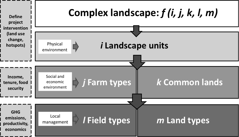
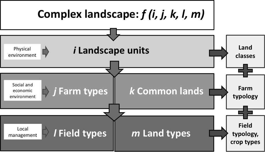
The targeting approach stratifies landscapes of different complexity into different classes, to identify units that provide estimates of emissions reductions representing larger areas. Figure 2.1 shows how a complex landscape can be split — using a top down approach — into smaller units (i landscape units) that have a common biophysical environment at regional scale. This disaggregation can be done using GIS and RS, assisted by existing secondary data. Landscape units can be further disaggregated into j farm types and k common lands to describe differences in the ways that individual households and communities access and use the land. The sort of units that link the land to land users will vary according to tenure systems in different territories, jurisdictions and countries (Ostrom and Nagendra 2006). This step uses information on incomes, land tenure and food security. It enables mitigation practices to be designed that are appropriate for heterogeneous rural communities, and where the land can be privately and communally managed. To make a connection with farming activities and ultimately with the level at which mitigation practices are implemented, farms and common lands can be disaggregated into l field types and m land types. This distinction may fade out in countries where the land is intensively used independently of the tenure system. The identified units can be studied in terms of land productivity, economic outputs, carbon stocks, GHG emissions, and the social and cultural importance of farming activities for rural families.
2.3 Top-down approach
We illustrate the steps to split a complex landscape (of any size) into homogeneous units using GIS and RS information and socioeconomic surveys to study mitigation potential (Figure 2.1). This may be of interest, for example, where a carbon credit project is implemented, or if a district, province or other authority wishes to assess the mitigation potential of a number of agricultural technologies. Once the landscape boundaries are defined, one can disaggregate the complex landscape into different units. If the landscape boundaries are not delineated, the analyst may choose to select an area that is representative of the larger region in order to extrapolate results. The landscape can be analysed initially using a combination of RS and GIS. We suggest different approaches to disaggregate a landscape and decide where to conduct field measurements.
After selecting a landscape for assessment and developing a conceptual model of land use and land cover (LULC), the simplest method to identify landscape units is the exploration and visual interpretation of satellite imagery, preferably with the best available spatial resolution and observation conditions (e.g. peak of vegetation productivity). LULC classification (using object-based approaches and VHR imagery) and landscape classification (using RS vegetation productivity parameters) are more sophisticated methods of approaching a landscape. With visual interpretation, numerous landscape features can be characterized using physical (e.g. geomorphology, vegetation, disturbance signs) and human criteria (e.g. presence of population, land use, and infrastructure). This yields relatively large, homogeneous landscape units (e.g. describing the mosaic of land uses and land covers in an area). By comparison, automated LULC classification yields results at a much finer spatial scale. In most cases it maps the individual fields that make up a landscape. The process of automated LULC mapping involves:
1. Discriminating areas of general LULC types such as croplands or shrublands
2. Characterizing structural traits of all these types
3. Integrating areas and traits to identify homogeneous landscape units.
The two first steps require the composition of the landscape to be characterized (i.e. the areas under each of the field or land types according to Figure 2.1), and their spatial configuration (i.e. the arrangement of field or land types).
In landscapes with dominant smallholder agriculture, cultivated land can be easily recognized through the presence of regular plots with homogeneous surface brightness, and minor features such as ploughing or crop lines and infrastructure. In addition, the structural heterogeneity of cultivated areas can be assessed by the geometry of the fields (size and symmetry of the shapes), the presence of productive infrastructure and signs of disruption, such as woody encroachment within fields. Land under (semi-)natural vegetation can be characterized in terms of vegetation composition (share of trees, shrubs and grass), signs of biomass removal or presence of barren areas, and degradation (gullies, surface salt accumulation). Finally, in order to delimit landscape units, all descriptions should be integrated in an holistic manner using, for example, Gestalt-theory (Antrop and Van Eetvelde 2000) to identify and digitize potential discontinuities. This simple method has the potential to enhance the quality of broad-scale land-use studies, and can be performed using freely available imagery, like Google Earth, supported by on-line photographic archives such as ‘Panoramio’ or ‘Confluence Project’ (Ploton et al. 2012).
2.3.1 Landscape stratification: an example from East Africa
The Lower Nyando region of western Kenya, which is dominated by smallholder producers, provides an example of the proposed approach. The CGIAR Program for Climate Change, Agriculture and Food Security (CCAFS) promotes climate smart agriculture in this area. To develop and test our targeting approach, we used the three methods described above: 1) visual classification using VHR imagery, 2) LULC classification using object-based approaches and VHR imagery, and 3) landscape classification using medium to coarse resolution RS vegetation productivity parameters.
Visual classification using VHR imagery
This is a quick and relatively inexpensive visual approach for exploring landscapes. The largest costs are the acquisition of the VHR images. Based on a QuickBird® image from the dry season (1 December 2008), six landscape classes were identified (Table 2.1 and Figure 2.2). This initial classification can be used to test whether the units are indeed related to soil emissions and mitigation potential. The landscape classification is expected to reflect differences in land productivity and GHG emissions, because it captures inherent soil and vegetation variability.
Class delimitation criteria and mitigation opportunities are listed for each class in Table 2.1. The limits between the classes are determined by spatial changes in the detailed criteria. As expected, these changes can be abrupt or gradual, and the ability or experience of the mapper could lead to variable results.
The visual delineation may or may not coincide with regional biophysical gradients, as shown by a quick assessment of the topography of Nyando (Figure 2.3). In our case study, the highlands coincided with areas allocated to cash crops, while the lowlands included a continuum from subsistence crops to wooded natural land types. Delineating a landscape on the sole basis of topography may be inaccurate and/or incomplete, yet the use of a digital elevation model (DEM) is an inexpensive option to simplify landscapes.
Land use and land cover classification using object-based approaches and VHR imagery
The fine-scale analysis of actual land use and land cover (LULC) allows the interface between biophysical and human induced processes to be captured. The automated methods are more complex than the visual interpretation described previously and require digital processing of remote sensing imagery. VHR satellite imagery with pixel resolution <1 m can be used for semi-automatic (supervised) mapping of LULC in heterogeneous and fine-structured landscapes with sparse vegetation cover. To make optimal use of the rich information provided by the VHR data, object-based approaches are recommended. Compared to pixel-based approaches, object-based approaches permit the full exploitation of the rich textural information present in VHR imagery, as well as shape-related information. They also avoid ‘salt and pepper’ effects when classifying individual pixels. Figure 2.4 summarizes the main steps of such an approach.
Table 2.1 List of visual classes determined for the Nyando study region, Kenya.
| Class | Delimitation criteria | Mitigation opportunities | |
| A | Cultivated land dominated by cash crops | Presence of an agricultural matrix, i.e. extensive (> 70% of the area) and connected (few identifiable large patches) cover. Most plots (> 75%) are comparatively large and of similar size (~1 ha), regular-shaped (rectangular), and have a heterogeneous colour and brightness. Heterogeneity in this class originates from plough or crop lines, pointing to a crop cover. Presence of infrastructure (e.g. houses, storage places, etc.). No degradation signs (e.g. surface salt accumulation, lack of vegetation, gullies). | Agroforestry, fertilizer management |
| B | Natural vegetation | Presence of a matrix of any original vegetation type (forests, shrublands, savannahs). Trees or large shrubs are clearly distinguishable by their round shape or shadows in the images. | Halting land and tree cover degradation |
| C | Mixed natural vegetation and agricultural land | No single cover type reaches 70% of the area, and patches of crop, pasture, and natural vegetation are intermingled. | Agroforestry, livestock management |
| D | Cultivated land dominated by subsistence crops | Same as A, but most plots are smaller, of variable area and shape (rounded, elongated, irregular). In this class, heterogeneity comes in addition from patches of herbaceous or shrubby vegetation within plots (a sign of land abandonment), and surface degradation. | Fertilizer and manure management, agroforestry |
| E | Agricultural land dominated by grazing land | Same as A, but most plots are comparatively larger, have irregular shape (no bilateral symmetry), and lack of plough or crop lines. Frequent isolated trees or shrubs inside plots. Signs of infrastructure are less common than in A. | Livestock management, manure management, agroforestry |
| F | Mixed cultivated land | Both elements of A and D are found intermingled within small areas. | Agroforestry, fertilizer and manure management |
In a similar way to Figure 2.2, the landscape is first segmented into small, homogeneous subunits or objects. This process is indicated in Figure 2.4 as image segmentation. Input to this image segmentation are geo-rectified, multi-layer very high resolution (VHR) satellite images. The resulting objects (also called “segments”) are groups of adjacent pixels, which share similar spectral properties, and which are different from other pixels belonging to other objects.
To segment a landscape using VHR satellite images, so-called segmentation algorithms are used. Contrary to the visual classification approach, objects/segments are identified in a fully automated manner. Both commercial and open source solutions exist for this task. Excellent open source solutions are, for examples, QGIS (www.qgis.org/), GRASS GIS (grass.osgeo.org/) and ILWIS (www.ilwis.org/).
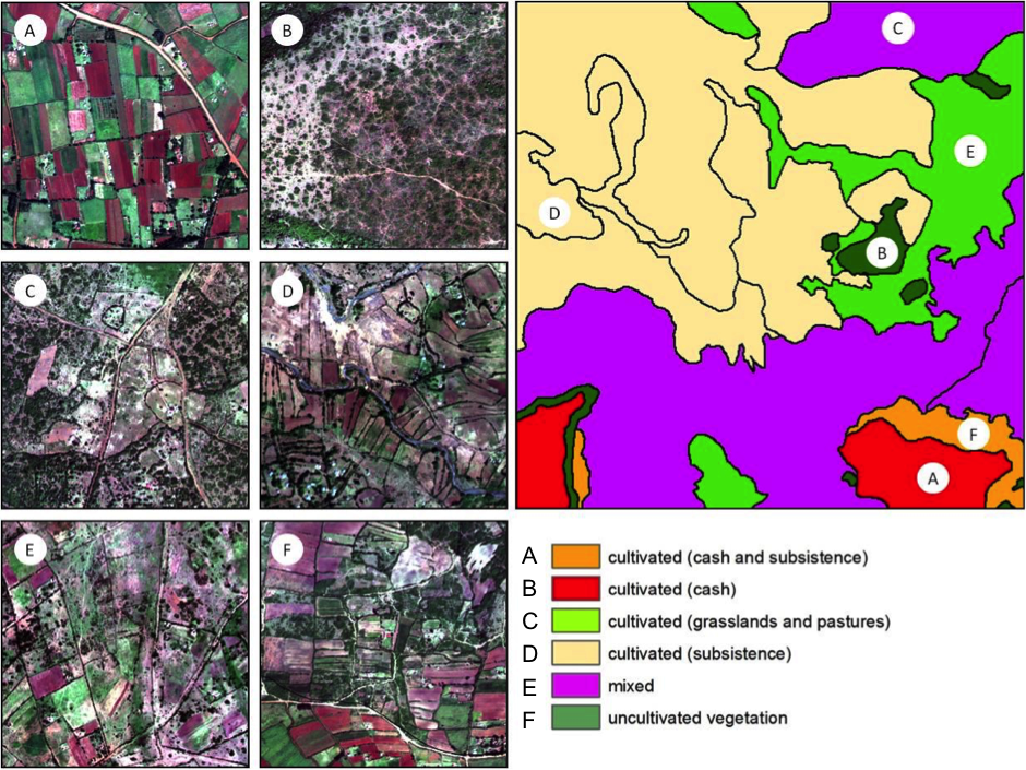 Fig. 2.2 Landscape analysis based on a visual inspection of landscape structure of Nyando, western Kenya. A–F are samples of the territory represented by the original QuickBird® image (all have the same spatial extent of 500 m). The larger panel on the right represents the six meaningful classes of landscape from the visual classification approach. Letters (A, B, C, D, E and F) show the location of samples in the area (see explanations in Table 2.1).
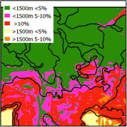
Fig. 2.3 Topographic characteristics of Nyando region. Altitude (masl) and slope (expressed as percentage) came from the Shuttle Radar Topography Mission (SRTM) digital elevation model (USGS 2004). The lines delineating the landscape units of Nyando are the same as in Figure 2.2.
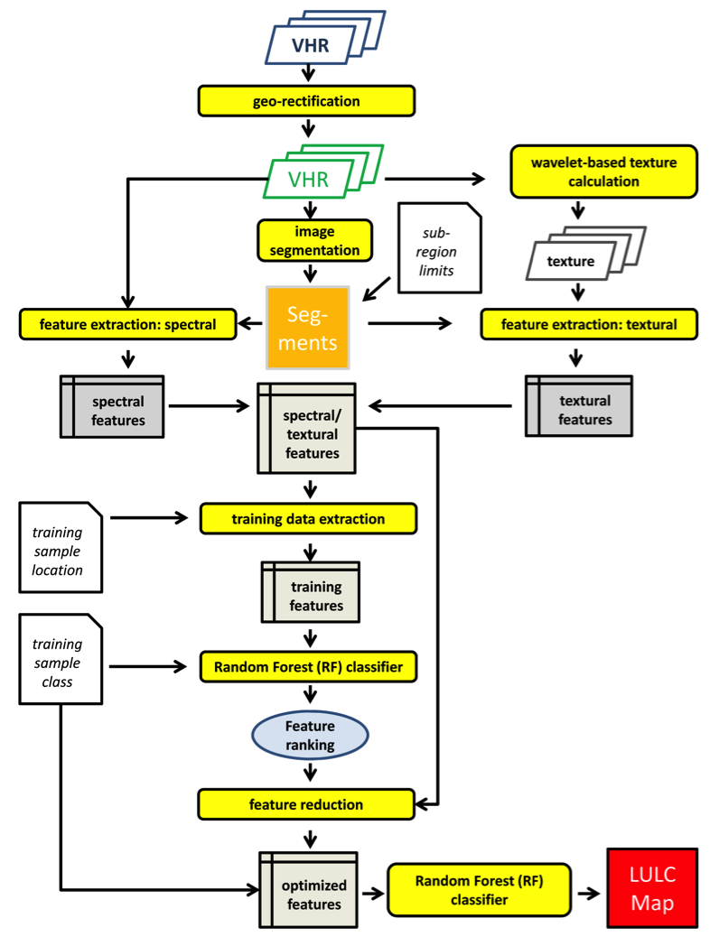
Fig. 2.4 Flowchart for object-based supervised classification of VHR imagery. The process yields a detailed LULC map of the area covered by the VHR satellite imagery, as well as information on the uncertainty of the classification outcome for each image object.
After segmenting the image into image objects, an arbitrary number of features are extracted for each object. In Figure 2.4 this process is labelled as feature extraction. Besides spectral features, textural features, as well as shape information, can be extracted. This information is used in a subsequent step to automatically assign each object to one of the user-defined LULC classes (process labelled as Random (RF) forest classifier). To ‘learn’ the relationship between input features and class labels, training samples with known LULC must be provided in sufficient numbers and quality using a process called training data extraction.
Because the relation between input features and class label may change depending on image location (e.g. related to terrain and elevation), a stratified classification is recommended. For this task, before starting the classification process, the entire scene is (visually) split into a few (larger) regions (or strata) that can be considered homogeneous in terms of land cover characteristics and the physical setting of the landscape.
The stratification is usually done just after the automated image segmentation (Figure 2.4). Of course, results from other studies can be used as well (e.g. boundaries shown in Figure 2.2). Figure 2.5a shows the RGB composite of a WorldView-2 image of the Nyando study area, and Figure 2.5b the corresponding DEM. In both maps, manually drawn landscape boundaries (strata) are also shown (yellow lines).
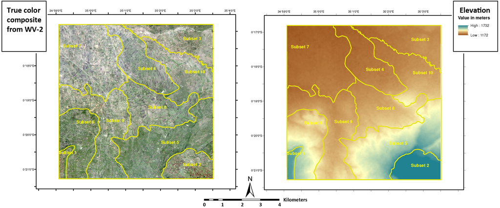
Fig. 2.5 Visualization of important steps of the supervised classification of the Nyando study region. (a) RGB image of WorldView-2® VHR imagery with manually delineated strata, (b) DEM of the region with strata.
For one of the strata, Figure 2.6a shows the available reference information obtained from fieldwork and complemented through visual image interpretation. These training samples are necessary for the RF classifier to ‘learn’ the relationship between input features and class labels. The resulting object-based classification is shown for this landscape unit in Figure 2.6b. The object limits (e.g. grey lines in Figure 2.6a) have been automatically derived using GRASS GIS.
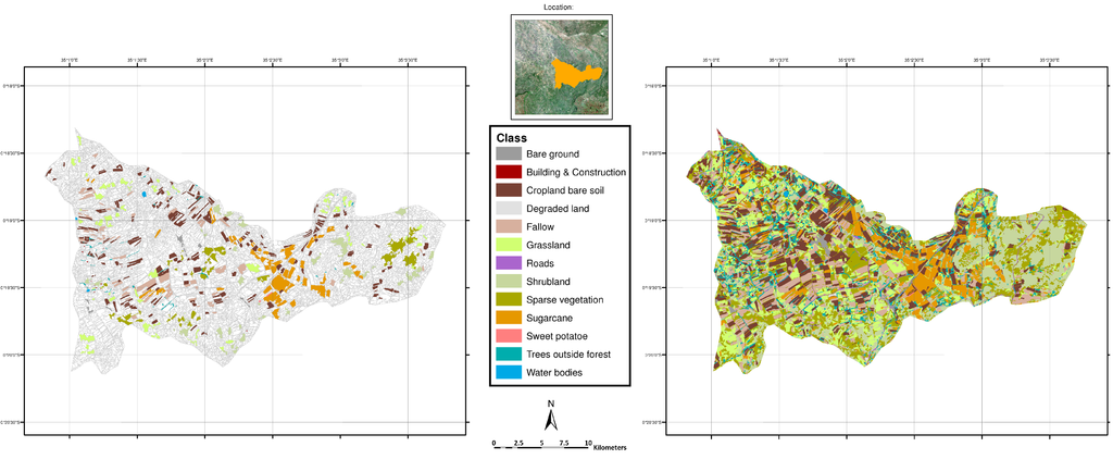
Fig.2.6 (a)Insituinformationabouttheland-use/land-coveroftrainingsamplesforoneofthe ten strata; the segmented image objects are also visible in gray, (b) classification result based on spectral and textural features of the WorldView-2® VHR image for the same stratum.
For the classification, several algorithms are available (e.g. maximum likelihood classifier, CART, kNN, etc.). Based on the authors’ own and published experience, we exploited a widely used ensemble classifier called ‘random forest’ (RF) which often yields good and robust classification results (Gislason et al. 2006, Rodriguez-Galiano et al. 2012a, Toscani et al. 2013). RF uses bootstrap aggregation to create different training subsets, to produce a diversity of classification trees, each providing a unique classification result. For example, if 500 decision trees are grown inside the RF, one will obtain 500 class labels for each object. The final output class is obtained as the majority vote of the 500 individual labels (Breiman 2001). The proportion of votes of the winning class to the total number of trees used in the classification is a good measure of confidence; the higher the score, the more confident one can be that a class is correctly classified. Similarly, the margin calculated as the proportion of votes for the winning class minus the proportion of votes of the second class indicates how sure the classifier was in their decision. Such confidence indicators are not readily obtained using visual image interpretation. RF also produces an internal unbiased estimate of the generalization error, using so-called ‘out-of-bag’ (OOB) samples to provide a measure of the input features’ importance through random permutation. Classification performance of the entire LULC map can be based on common statistical measures (overall accuracy (OA), producer’s accuracy (PA) and user’s accuracy (UA)) (Foody 2002) derived from the classification error matrix, using suitable validation samples. Figure 2.7 shows the resulting LULC map of Nyando obtained with this object-based classification approach and using VHR imagery from WorldView-2®.
Landscape classification using RS vegetation productivity parameters
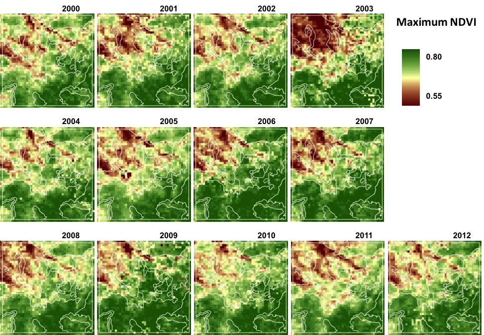
The two previous approaches are based on static descriptions of the landscape units (or of their constituent elements) in terms of LULC. However, alternative land traits can be explored to determine homogeneous landscape units. A promising alternative is the analysis of vegetation function in terms of the magnitude and temporal variability of primary productivity (Paruelo et al. 2001). We tested this functional analysis in Lower Nyando, using the period 2000–2012. Vegetation primary productivity was assessed through the proxy variable Normalized Difference Vegetation Index (NDVI). This index has been of great value for biogeographical studies, allowing rough but widespread characterizations of the magnitude and temporal variability of productivity based on homogeneous measurements across wide spatial and temporal extensions and different ecosystems (Lloyd 1990, Xiao et al. 2004, Sims et al. 2006). In this example, we acquired NDVI data from the MODIS (Moderate Resolution Imaging Spectroradiometer) Terra instrument. In this data set, one image is produced every 16 days, leading to 23 images per year.
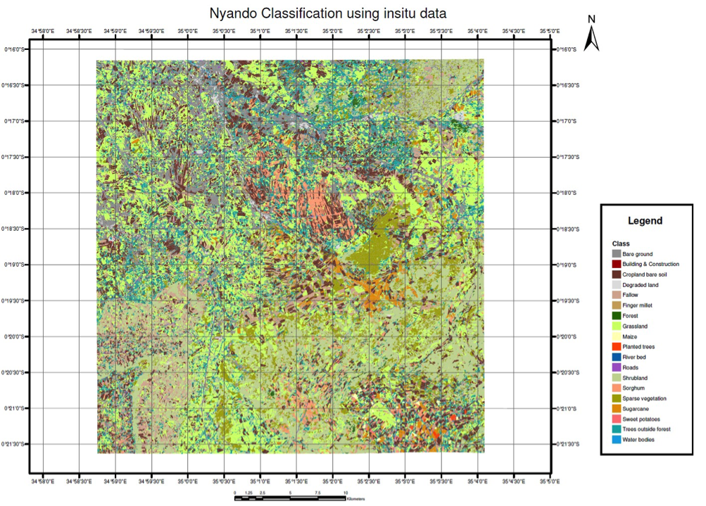 Fig. 2.7 LULC map of Nyando from WorldView-2® VHR imagery, using an object-based classification approach
We selected from the 13-years x 23-dates database, only those values indicating good to excellent quality conditions (i.e. pixels not covered by clouds, and with a low to intermediate aerosol contamination). Then, we used the code TIMESAT v.3.1 to reconstruct temporal series (Jönsson and Eklundh 2002, Jönsson and Eklundh 2004, Eklundh and Jönsson 2011). This tool fits smoothed model functions that capture one or two cycles of growth and decline per year. We selected an adaptive Savitzky-Golay model (Jönsson and Eklundh 2002), assuming two vegetation growth cycles per year due to the natural bimodal behaviour of rains in the study region. From the reconstructed temporal series (and by means of TIMESAT and the R v.2.15 statistical software), we calculated different functional metrics depicting average annual magnitude (e.g. mean, maximum NDVI) and seasonality (e.g. coefficient of variation (CV) of available values, number of growing seasons), and interannual variability (e.g. CV of mean annual values, annual trends) (Baldi et al. 2014).
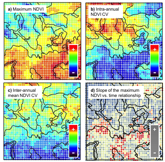
For the sake of simplicity in the Lower Nyando example, Figure 2.8 presents: a) NDVI maximum values as a proxy for carbon stocks of cultivated and uncultivated ecosystems; b) intra-annual CV, describing whether the productivity is concentrated in short period or distributed evenly through the year; c) interannual CV of mean annual values, describing long term productivity fluctuations; and d) the slope of the maximum annual NDVI versus time relationship (Paruelo and Lauenroth 1998; Jobbágy et al. 2002).
Figure 2.9 shows the entire temporal range for the case of maximum annual values. Combined, structural and functional assessments provide essential information about the quality of the detected field or land types to study GHG mitigation potentials. Likewise, this approach may reveal functional divergences between a single field or land type, or convergences between different classes as shown in Figures 2.8 and 2.9, with strong impacts on cascading ecosystem processes.
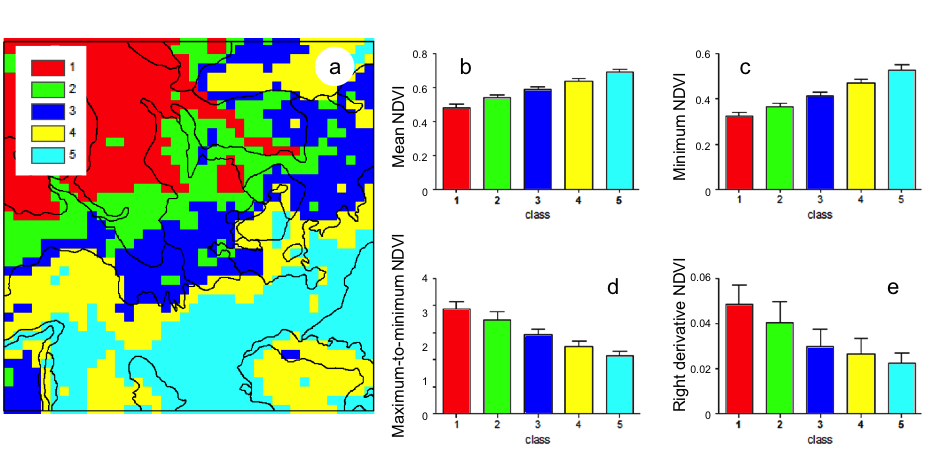
To identify landscape units using only functional information, we integrated functional attributes by applying an unsupervised classification procedure. In contrast with a LULC classification, we do not expect a priori conceptual scheme, both in terms of the number of classes and their identity. Functional classes often have to be split or merged to create a meaningful map, i.e. to show patterns of patches and corridors rather than isolated pixels (‘salt and pepper’ appearance). Using the unsupervised clustering algorithm ISODATA (Jensen 1996), we generated a map delimitating five different classes which reached our pattern-based expectations (Figure 2.10). This approach revealed functional divergences between single farm types or common lands (e.g. western versus eastern cultivated areas dominated by cash crops), and convergences between different classes (e.g. western mixed shrubs and cultivated land versus eastern cultivated areas dominated by cash crops), with potential impacts on cascading ecosystem processes.
In addition to the landscape analysis, other on-the-ground information is needed for the development of a representative sampling design for smallholder systems before resource-consuming measurements of soil GHG fluxes or soil carbon and nitrogen stock inventories are implemented. The characterization of farmers’ socioeconomic condition is important here, because this also affects resource management. On-farm variations in soil properties, which result from long-term differences in field management, create soil fertility gradients that may justify the use of a field typology.
2.4 Bottom-up approach
For some specific landscapes or agricultural systems there may be a wealth of field data that characterize the use of the land at field and farm level. This could include household surveys, soil surveys, productivity and economic assessments. This information comes at the price of laborious and costly data collection, and we encourage scientists and project developers to take advantage of existing field and farm data to inform the targeting of mitigation options at the local level. The analysis of these data inform the selection of field and farm types indicated in Figure 2.1, which are the ultimate entry point for deciding where to carry out GHG measurements and identifying mitigation practices. This field level characterization is especially useful in very fragmented landscapes, where topography, soils and long-term management create strong gradients in soil fertility and water retention capacity, which may lead to differences in emissions potential (Yao et al 2010, Wu et al 2010). We acknowledge that such detailed characterization may not be needed in simple landscapes with few land uses and relatively flat relief. Expert opinion by soil scientists can help decision-making about the location of field level assessments.
We present a method that can be used to link the fields and farming practices with the landscape level, and emissions due to agricultural practices with potential for emissions reductions at scale. The method is based on assumptions 2 and 3 presented in Section 2.1: i.e. that the diversity of soils and land management can be meaningfully summarized using a field typology, which connects farmers’ fields to landscape units representing inherent land quality and human-induced changes. There is evidence that field types can be defined on the basis of simple indicators that are correlated to land quality and land productivity. Research in western Kenya and Zimbabwe shows the relationship between soil quality, intensity of management and land productivity (Tittonell et al. 2005, Tittonell et al. 2010, Zingore et al. 2007), which we believe are correlated to soil GHG emissions.
A field typology can be derived a priori using information collected in household surveys. This can help connect field management with farm types, defined by livelihood indicators, including food and tenure security. Including these dimensions in the analysis provides an opportunity to link mitigation with food security and poverty to estimate trade-offs and synergies. Such an analysis permits an assessment of the feasibility of mitigation for different farmers and identification of the incentives needed for adoption. Land users can assess and weigh up the livelihood benefits of different practices (e.g. income, increased production of food) and the costs of implementing such practices.
Using the Lower Nyando site, we show how to use household and field surveys to support targeting at a local level and how to link it to the selected landscape. We collected existing information on households and farm management. The lower Nyando site was characterized using the IMPACTlite tool (Rufino et al. 2012a,b) that gathered generic data to analyse food security, adaptation and mitigation in smallholder agriculture. A comprehensive household survey was conducted to characterize household structure, asset ownership, farm production, costs and benefits of farming activities, other sources of income generation, and food consumption (Rufino et al. 2012 a,b). Using the farm household characterization, and to elaborate the field typology, fields recorded in the household survey were measured, geo-referenced and additional management data were collected. The household survey covered three production systems across the sampling frame of the Kenyan CCAFS site of Nyando (Förch et al. 2011), and included 200 households. A field typology was built on the basis of field type scores collected through a survey (see forms in Appendix 2.1). A subsample of fields was selected randomly to represent the field types.
2.4.1 Field Typology definition
The field typology must reflect inherent soil fertility resulting from soil type and long-term management. The process of defining the field typology is dependent on the landscape within which the project works and the sociocultural norms of the farmers. For example, crop diversity may be considered as a sign of productive land in subsistence agriculture systems. Adjusting the weighting to take into account local knowledge is important to link well with ground truths.
The scores obtained through this process are simply a tool for subdividing fields based on easily obtainable data, analogous to a rapid rural appraisal (Dorward et al. 2007). It is often justifiable to adjust the weightings based on the data, by identifying the common characteristics of the field types and checking that the subdivisions are indeed meaningful. Whenever possible the classification should be counter checked against the common sense evaluation of an experienced field officer on the ground.
At the Nyando site, we used a number of variables to define a field type score:
• Crop This score is the sum of the crops that each household is cultivating in one plot. Intensively managed fields are cropped with several crops, which often receive more agricultural inputs than other fields.
• Fertilizer use This score distinguishes organic and inorganic fertilizers. Manure was given a score of 2 and other inorganic fertilizer a score of 2. It was assumed that fields receiving inorganic fertilizers are managed more intensively than fields that only receive animal manure.
• Number of subplots This is the number of subplots within a given field or plot. Subplots are units within a field or permanent land management structure that can change in space or time. This aims to capture the spatial and temporal allocation of land to crops, crop mixtures, and the combination of annual and perennial crops in intercropping, permanent and seasonal grazing land.
• Location of field Fields next to the homestead receive a score of 2, while fields further away from the house receive a score of 0. This assumes that fields close to the homestead receive preferential land management (e.g. fertilization, addition of organic matter, weeding) compared to fields that are far away.
•Signs of erosion Fields differing in visible signs of erosion obtained different scores, depending on severity. For gulley, rill and gulley/sheet/rill erosion, fields received a score of 0. Sheet erosion or no visible erosion obtained a score of 1.
Plots with a score higher than 10 were labelled as field type 1. Those with scores between 4 and 10 were labelled as field type 2, and those with scores lower than 4 were labelled as field type 3. The process of defining scores for each variable involved making judgments about correlations and data quality. The end scores were then investigated, definitions adjusted and natural cut-off points identified. The identification of natural cut-offs for the field types is a delicate process because the scoring tool is crude enough that one would not expect a substantial difference on the ground between borderline cases. A useful guideline is that borderline cases should not be either under- or over- represented in any field type.
2.5 Combining top-down and bottom-up: the basis for scaling up
The field typology sampled across households represents the diversity of land management practices. If it is combined with a land-use classification, it connects local management with landscape characteristics as indicated in Figure 2.11. Provided that land-use units or land classes have been sampled at field level, or that spatially explicit information is available on the diversity of field types, connecting these two layers may provide a measure of variability on GHG emissions, productivity and livelihood indicators. To achieve this, enough field sites have to be selected to represent each landscape class, and must be monitored for GHG emissions, carbon stock changes, production of biomass and other variables of interest. The number of replicates or field sites to represent a landscape class will depend on within-class heterogeneity, and the resources available for monitoring emissions. An absolute minimum of three replicates per land class is required to estimate biophysical parameters.
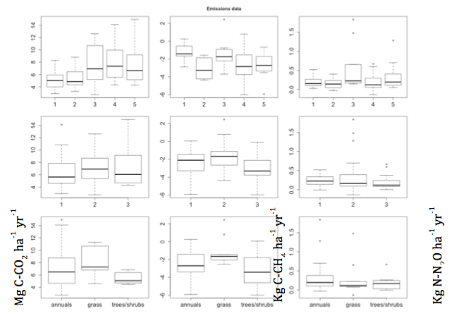
The advantage of selecting replicated field sites that correspond to landscape classes is the possibility to scale up (i.e. to estimate project-level benefits and trade-offs with livelihood indicators). It also provides an opportunity to extrapolate findings to similar environments. In the case of lower Nyando, we combined the field typology derived from a household characterization with the landscape description including five classes or units shown in Figure 2.10. ‘Landscape plots’ were selected to represent field types using landscape units where we monitored GHG emissions, analysed carbon stocks, and estimated productivity and the economics of production. We present here the results of 12 months of monitoring GHG emissions aggregated at field and landscape level (Figure 2.12). The information provided a comprehensive database to estimate emissions potential and trade-offs with other socioeconomic indicators, such as income and land productivity. Additional fields sites were added to compensate for areas poorly represented by the household survey and to include natural areas. This can be a serious disadvantage of using secondary data in a bottom-up approach, where householders neglect natural areas such as woodlands or wetlands during interviews. Natural areas were selected from the landscape analysis, where natural vegetation units were mapped.
2.6 Conclusions
A methodology is presented to target mitigation research at field, farm and landscape level. It uses both a top-down and a bottom-up approach to capture local diversity in soils and management practices, and landscape heterogeneity. It enables generic recommendations to be made about scaling up alternative mitigation options. The methods can fit the purposes of diverse projects, including the targeting of GHG measurement or the testing of carbon sequestration practices. The products generated such as land-use or land class maps and selected field types allow field sites to be selected for monitoring biophysical parameters. Once monitoring of GHG emissions, productivity and economics are finalized, the nested approach suggested here provides a basis for scaling up, which can be achieved using different analytical methods discussed in Chapter 10 of this volume.
Author affiliations
¹Lancaster Environment Centre, Lancaster University, formerly Center for International Forestry Research (CIFOR), Nairobi, Kenya
2 University of Natural Resources (BOKU), Peter Jordan Strasse 82, 1190 Vienna, Austria
3 Instituto de Matemática Aplicada San Luis, Universidad Nacional de San Luis and Consejo Nacional de Ciencia y Tecnología (CONICET). Ejército de los Andes 950, D5700HHW. San Luis, Argentina.
4International Livestock Research Institute (ILRI), PO Box 30709, Nairobi, Kenya
5Karlsruhe Institute of Technology, Institute of Meteorology and Climate Research, Atmospheric Environmental Research (IMK-IFU), Kreuzeckbahnstr. 19, Garmisch-Partenkirchen, Germany
6World Agroforestry Centre (ICRAF), PO Box 30677, Nairobi, Kenya
7Maseno University, PO Box 333, Maseno, Kenya
References
Breiman L (2001) Random forests. Mach Learn 45:5-32.
Eklundh L, Jönsson P (2011) Timesat 3.1 Software Manual. Lund University, Lund, Sweden
Jensen JR (1996) Introductory Digital Image Processing: A Remote Sensing Perspective, Pearson Prentice Hall, New Jersey, USA
Pelster DE, Rufino MC, Rosenstock TS, Mango J, Saiz G, Diaz-Pines E, Baldi G, Butterbach‐Bahl K (submitted) Smallholder African farms in western Kenya have limited greenhouse gas fluxes. Global Biochemical Cycles.
Rufino MC, Quiros C, Teufel N, Douxchamps S, Silvestri S, Mango J, Moussa AS, Herrero M (2012b) Household Characterization Survey – IMPACTlite Training Manual. Working document, CGIAR Research Program on Climate Change, Agriculture and Food Security (CCAFS), December 2012
Appendix 2.1