Methods for smallholder quantification of soil carbon stocks and stock changes

Gustavo Saiz¹ and Alain Albrecht²

Abstract Smallholder agricultural systems in tropical and subtropical regions may have significantly contributed to greenhouse gas (GHG) emissions over the past number of decades. As a result, these systems currently offer large GHG mitigation potentials (e.g. soil organic carbon (SOC) sequestration), which can be realized through the implementation of good management and sustainable agricultural practices. In this chapter we synthesize current available methodologies designed to assess SOC stocks and stock changes. From this analysis, it becomes apparent that the design and subsequent implementation of any quantification and monitoring scheme envisaged for studies focusing solely on the soil component greatly differs from those developed for whole ecosystem accounting, not just in its approach, but also in the amount of resources needed to implement it within a given degree of accuracy. We provide analyses and recommendations on methods specifically dealing with quantification and assessment of SOC at both the individual farm and the landscape scale in smallholder agricultural systems.

Summary Video in English or French

7.1 Introduction

Agricultural activities are responsible for about one third of the world’s greenhouse gas (GHG) emissions and this share is projected to grow, especially in developing countries (IPCC 2007). Indeed, smallholder agricultural systems are highly dynamic and heterogeneous environments that may have significantly contributed to GHG emissions over the past number of decades (Berry 2011). Furthermore, these systems traditionally suffer from severe soil organic matter (SOM) depletion due to intense decomposition following soil ploughing, the removal of most of the aboveground biomass during harvest, and the enhanced soil erosion inherent to those activities. Yet, they may also offer large mitigation potentials through the implementation of good management and sustainable agricultural practices, particularly through improvements in land-use management, as nearly 90% of IPCC-identified technical potential lies in enhancing soil carbon sinks (Lipper et al., 2011).

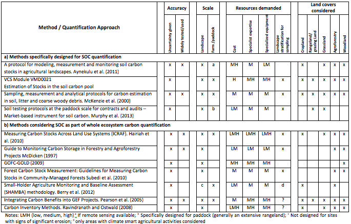
A number of methodologies are currently available for the quantification of carbon stocks in terrestrial ecosystems, varying widely in terms of accuracy, scale and resources needed for their implementation (e.g. Pearson et al., 2005; Ravindranath and Ostwald, 2008; Hairiah et al., 2010). Table 7.1 offers a comparative analysis of methods for quantification of soil organic carbon (SOC) stocks and changes with regard to level of accuracy, scale, resources demanded, and land covers considered. While nearly all the schemes feature soil as a component of the total carbon pool, the number of methods specifically designed to assess SOC stocks and stock changes are considerably more limited This is despite the wide acknowledgement that many ecosystem services are strongly correlated with SOC levels, and their huge importance for sustaining local livelihoods. The design and implementation of any quantification and monitoring methodology for studies focusing solely on the soil component may greatly differ from those developed for whole ecosystem accounting, not only in approach or the accuracy but also in necessary resources. Therefore, it is justified to develop methods that can effectively deal with soil carbon quantification and monitoring for a given accuracy within the available budget. In the present work we focus on the soil component and provide analyses and recommendations for methods to quantify SOC in smallholder agriculture in tropical environments.

The SOC inventory in a given soil profile is controlled by the complex interaction of many factors, including climate, soil texture, topography, fire frequency, land use and land management (Bird et al. 2004; Saiz et al. 2012). These drivers exert contrasting influences on SOC stocks at different spatial scales. At the local scale, biotic factors and management activities play a fundamental role in affecting the quantity and quality of carbon inputs and decomposition processes, while at larger scales the variation in SOC stocks is mainly controlled by topographic, edaphic and climate related factors (Wynn and Bird 2007; Allen et al. 2010; Saiz et al. 2012). Ultimately, an increase in SOC levels at a given site may occur either through the reduction of factors promoting SOM mineralization and lateral exports (e.g. erosion), and/or by increasing SOM inputs and enhancing stabilization mechanisms (e.g. physical protection of SOM through stable aggregates).

Table 7.1 Comparative analysis of methods for smallholder quantification of SOC stocks and changes with regard to level of accuracy, scale, resources demanded, and land covers considered

Given the inherent high spatial variability of SOC, accurate quantification and monitoring of SOC stocks and stock changes is a complex task even in relatively homogeneous ecosystems. This complexity is further exacerbated in smallholder environments by the existence of multiple land use activities occurring at various management intensities. Moreover, sources of uncertainty and suitable levels of precision and accuracy differ when working at the landscape scale as opposed to the farm scope because biogeochemical processes affecting SOC dynamics operate and interact at different spatial scales (Veldkamp et al., 2001; Milne et al., 2013). Therefore, efficient sampling designs are needed across smallholder agricultural systems to ensure that SOC stocks and stock changes can be detected at various scales for a given accuracy and at minimum costs (Milne et al., 2012; Singh et al, 2013). Chapters 2 and 3 in this book provide some critical discussions on sampling designs specific to smallholder contexts. These chapters deal with systems characterization and targeting, and determination greenhouse gas emissions and removals associated with land use and land cover change.

In the present work, we propose an integrated field based approach for small household systems that encompasses estimates of SOC stocks and stock changes both at farm and landscape scales over a wide range of land use management intensities.

7.2 Quantification of soil carbon stocks

7.2.1 Sampling design – stratification of the project area

While the establishment of a geographical extent for quantification of SOC stocks and stock changes at the farm level can be straightforward, it is not the case for smallholder landscape assessment. The landscape concept may be defined by a geographic or ecological boundary, which often includes a mosaic of land covers and land uses that are managed in several different ways by the multiple stakeholders involved. In this context, Chapter 2 in this book provides recommendations for stratifying the landscape according to its agricultural productivity, economic outputs, potential GHG emissions, and social and cultural values. A SOC quantification scheme could integrate with such a stratification approach at the landscape level.

Herein, we describe the methods specifically dealing with quantification and assessment of SOC at both the individual farm and the landscape scale in smallholder agricultural systems.

Farm level Intensive work conducted over the past decade in smallholder agricultural systems in sub-Saharan Africa has demonstrated the existence of within-farm variability of soil fertility and related soil properties (Prudencio 1993; Carsky et al. 1998; Tittonell et al. 2005a; 2005b; 2013). A common feature of these farming systems is the existence of strong gradients of decreasing soil fertility with increasing distance from the homestead, which mainly occur as a result of differential resource allocation driven by the farmer. This spatial gradient must be taken into account when designing SOC sampling strategies in these agricultural systems, and more so considering that previous work has also identified strong correlations between yields, soil quality indicators, land use management and the distance from the homestead (Tittonell et al. 2005b; 2013). On the other hand, the presence of either annual or perennial vegetation on a given land use may have a strong impact on SOC stocks, as they significantly determine both the quantity and quality of organic matter inputs into the soil (Guo and Gifford 2002; Saiz et al. 2012). Therefore, distance from the homestead and land use classified by presence of annual or perennial vegetation, are the main criteria to use in order to categorize field types for the purpose of soil sampling. Accordingly, fields are classified into home gardens, close-distance, mid-distance, and remote fields following a similar procedure as in Tittonell et al. (2005b). These areas may contain several land uses, and as it may not be feasible to sample all of them, priority should be given to the actual representativeness of the land uses being considered. Therefore, sampling should be preferentially done in the largest fields provided that management activities with potentially heavy impact on SOC stocks, such as manure additions or recurrent burning of stubble, are roughly comparable between the different land uses. However, this assumption may not hold quite true in these farming systems, and thus it is worth noting that if land use management needs to be adequately quantified, then the sampling effort may need to be increased quite considerably. Nonetheless we hypothesize that, on the whole, soil sampling across a spatial gradient may partially account for the effect of land management intensities along the farm, given that such activities are also likely to occur along the same gradient.

Landscape level Assessment of SOC stocks at the landscape scale can be done following a spatially stratified randomized sampling design, as this will allow for a more optimum areal coverage and unbiased assessment of sample mean, variance and estimation variance of the sample mean. At the landscape level, the stratification can be done either through: a) ancillary data, or b) geographic coordinates, which may include the use of a systematic grid over the project area (de Gruijter et al. 2006).

Stratification through ancillary variables requires the establishment of discrete strata on which selected factors affecting SOC stocks show some degree of uniformity. Once the study boundaries have been defined, the use of remote sensing in combination with geophysical and management information may provide an effective means to stratify the target area (Ladoni et al. 2010). Such stratification needs to be performed considering, at minimum: available soil classifications, soil texture, landform information, topographic position, land cover, land use, management history, fire records, and obvious soil erosion/deposition processes. The initial stratification should be conducted in a hierarchical order whereby the factor that exerts the strongest influence on SOC stocks is ranked first, and other factors with less influence on SOC are subsequently assigned (e.g. a classical ranking approach might be climate, soil texture, land cover and management, etc.). The VCS module (VMD0018) provides detailed methodology on how to implement and adapt the stratification to the needs of the sampling process. Ideally, the number of samples to be measured in each stratum should be determined as a proportion of the area and the variance observed for that particular stratum. For this, a pilot soil sampling can be conducted which would serve a double purpose: to obtain an initial estimate of the variance for each stratum and serve as a training exercise for technicians who will be involved in subsequent sampling (MacDicken 1997). Nonetheless, it is likely that in smallholder systems, a stratum defined by biophysical factors may still be made up of land parcels managed in highly contrasting ways. Indeed, land management could account for more variation in SOC stocks at the landscape/ regional level than either soil types or land use. Under such circumstances, there may be a need to stratify into a greater number of land use categories to account for land use management practices between farm tenancies (Bell and Worrall 2009). Consequently, the number of samples needed to account for spatial patterns and uncertainty in a highly heterogeneous environment can quickly become impractical due to the cost and time associated to sample collection, preparation and analyses. To avoid this, spatially stratified systematic sampling approaches such as the one employed by the Land Degradation Surveillance Framework (LDSF; Aynekulu et al. 2011; Vågen et al. 2015) are easier to establish and monitor, and therefore may be a cost-effective alternative to provide a representative landscape estimate of SOC stocks and their changes. Moreover, the resulting sampling locations are spatially dispersed across the study area, but the range of variation in SOC stocks is not as effectively covered as with the stratification by ancillary variables. Therefore, the user should make his/her own choice depending on the available resources and the degree of accuracy required. We advocate the stratification by ancillary variables. However, in the case of very large heterogeneous regions, we recommend the implementation of a spatially stratified systematic sampling. It is worth stressing that while both stratification approaches (spatial and using ancillary variables) can yield relatively accurate information about SOC stocks at the landscape level, they lack proper accounting at the farm scale unless specific sampling strategies within a given household are further implemented.

The number of plots required to estimate SOC stocks in each stratum depends on the desired precision, often set at ±10% of the mean at 90 or 95% confidence level. The number of plots per stratum can be ascertained through the relationship described by Snedecor and Cochran (1967); See specifics in the detailed methodology section (Appendix A).

An initial soil sampling campaign should be conducted to establish baselines that can be used as references to monitor changes in SOC stocks. The level of precision required for a SOC inventory will undoubtedly influence the number of plots to be sampled, which will have necessarily a very strong impact on the cost associated with fieldwork and soil processing. Indeed, the largest component of the total cost incurred in SOC surveys corresponds to soil sampling and preparation (Aynekulu et al. 2011). Except for the case of surveys in which extremely large numbers of samples are collected (>2000), the actual cost of soil analyses is relatively low compared to the total expenditure derived from the collection and preparation of samples. Withal, and in order to minimize the number of samples to be analysed, an extensively applied method is the bulking (pooling) of samples collected within a plot at the same depth interval. This procedure has been shown to be a cost-effective technique for smoothing out local heterogeneity and for achieving robust local and regional estimates of SOC inventories (Bird et al. 2004; Wynn et al. 2006; Saiz et al. 2012).

The specific objectives of the study shall ultimately dictate the sampling priorities, which combined with the available resources, will determine the methodology and sampling intensity to apply.

7.2.2 Sample collection

Ideally, samples undergoing analyses should be as representative as possible of the area of interest. To help with this, samples can be combined to provide a single representative composite sample, but there should be at least several composite samples per selected plot to provide an estimate of variance. Therefore, we propose to take three soil samples (which will be subsequently pooled by depth interval before analyses) at four locations in each plot. A plot will correspond to a given field and land use within each selected farm. The initial sampling location will roughly be allocated at the centre of the field, with three replicates laid out according to a pattern of three axes separated 120 degrees with respect to an initial axis pointing north. The replicates will be selected along these axes at approximately mid distance between the centre of the field and its boundaries. The final sampling locations will be geo-referenced using a GPS, and notes should be taken about the sampling location with regard to the proximity of perennial vegetation (i.e. shrubs, trees, etc.), and any other relevant information such as presence of rock outcrops. Unless very intensive sampling is required in a given particular field, then the low analytical load proposed at the field scale (four composite samples) does not allow for proper inter-comparison of small-scale intercropping, or for comparison between furrows and ridges. Therefore, sampling should be systematically allocated at the same ploughing feature (e.g. furrow).

Previous to any sampling surface litter will be removed by hand. Soil samples will then be collected at 0-10 and 10-30 cm depth intervals making use of a steel corer. This procedure will allow for determinations through the retrieval of a single soil core of both OC abundance and accurate soil bulk density (SBD) at each depth interval. Accurate determination of SBD in the topsoil layers is particularly critical given that it is at these shallow locations where SBD shows the largest variability and significantly large quantities of OC are stored. Nevertheless, it is important to note that while the use of a steel corer may be a feasible procedure in many arable lands as a result of both soil being regularly disturbed and stones being progressively removed over the years, the use of a soil auger may be necessary to collect samples in stony or very hard soils. Indeed, impenetrable layers permitting, soil sampling at 30-50 cm needs to be carried out individually at each of the four sampling locations. In this case, replication at each sampling location is avoided because of the considerable extra time and effort that would be required. Section 7.2.4 explains the different procedures that can be used to calculate SOC stocks.

7.2.3 Sample preparation and analytical methods

(see also the Simplified Protocol for this purpose in Appendix B)

Once in the laboratory, samples are weighed in their sealed bags, clumps broken by hand and then oven dried at 40°C to constant weight. Thereafter, an aliquot of each sample will be oven dried at 105°C for 4 h which will allow for the calculation of soil bulk density (SBD), while the remainder of the samples will then be dry sieved to 2 mm and gravel and root content >2 mm determined by weight.

Standard methods of soil carbon analysis such as dry combustion or wet oxidation are extensively used in SOC studies as they provide optimum quality results. Moreover, elemental (dry) combustion appliances can be coupled to mass spectrometers to provide stable isotopic carbon signatures of SOM, which broadens the possibilities for better assessing soil carbon dynamics (Bird et al. 2004). However, the elemental combustion technique is resource-demanding and may be impractical or too expensive for large sets of samples and for continuous monitoring (Aynekulu et al. 2011; Batjes 2011). Nonetheless, the amount of time required to estimate SOC stocks and the sampling and analytical costs can be greatly reduced by employing emerging techniques for in situ estimation of SOC. Among such techniques the one that has been most widely used, and thus tested, is the Infra-Red Reflectance Spectroscopy, either at the Near or Mid infrared reflectance spectroscopy (NIRS or MIRS), which once calibrated can provide rapid accurate SOC estimates (Shepherd and Walsh 2002; 2007; Aynekulu et al. 2011). Despite its usefulness and versatility, it is still necessary that a significant proportion of samples (i.e. 20%) covering the projected range of SOC values for a given inventory are analyzed using standard SOC analytical procedures. This will in turn offers the necessary calibration set to confidently apply either MIRS or NIRS to the total set of samples. The use of remote spectroscopy on airborne or satellite-mounted sensors can also provide spatially distributed and resource-efficient measurement of SOC content (Ladoni et al. 2010). However, these techniques still require simultaneous ground observations to allow for proper calibration, and there are several major challenges associated with data accuracy (Croft et al. 2012; Stevens et al. 2006).

7.2.4 Quantification of SOC stocks

There are different approaches to account for soil carbon stocks and stock changes, and they all aim at providing a measure of mass of SOC per unit ground area.

The spatial coordinate approach calculates stocks considering the amount of carbon contained within a given volume of soil, which is defined by the sampled area and the depth referenced to the surface level. With this approach, the average SOC stock for a given depth interval (d) is calculated according to the following formula:

where:

μ_d is SOC stock (Mg OC ha^-1)

BD_d is soil bulk density (g cm^-3)

OC_d is the concentration of OC in soil (< 2 mm; mg OC g^-1soil)

D is soil depth interval (cm)

gr is fractional gravel content, the soil fraction > 2mm.

However, the amount of soil contained within a given volume (soil bulk density) may change as a result of swelling and/or compaction caused by land use change or management. Under those circumstances, sampling to a fixed depth from the surface (spatial coordinate approach) will result in different amounts of soil mass being sampled for the same volume, while the soil C concentration per unit dry soil mass might not have changed. This can lead to errors in the interpretation of changes in SOC storage following disturbance.

The determination of SOC stocks can also be achieved through cumulative or material mass coordinate approach, which consists of collection and quantification of all the soil mass in a given depth interval. The use of cumulative mass coordinate approach is widely used to correct for differences in bulk density that may have been caused by land use change or agricultural practices. Moreover, the adoption of this method may improve our ability to make comparative measurements across time, treatments, locations, and equipment (McKenzie et al. 2000; Gifford and Roderick 2003; Wuest 2009). Furthermore, since sampling by mass avoids potential biases derived from varying bulk density caused by land use change or agricultural practices, it is often regarded as the method of choice for SOC monitoring over time (see McKenzie et al. 2000 and Gifford and Roderick 2003 for detailed guidance on the method). Nonetheless, compared to soil coring, this method requires additional effort and skill. In the cumulative mass approach, depth varies such that each sample contains the same dry mass per unit ground area. Gifford and Roderick (2003) provide in-detail explanations and examples on how to determine SOC stocks using this methodology. Briefly, the method involves coring a bit deeper than the nominal depth involved (e.g. 55 cm for a required 50 cm depth) and each full soil core is then divided into several segments. We recommend sampling at 10, 30, 50 and 55 cm in those cases where coring may be feasible in order to compute for soil bulk density and be able to inter-convert between the spatial coordinate and the cumulative mass coordinate approach.

Another method that has been recommended to quantify SOC stock changes is the equivalent soil mass approach (Ellert and Bettany 1995; Lee et al. 2009). It consists of correcting for differences in SBD through the calculation of the mass of SOC in an equivalent soil mass per unit area (i.e. the heaviest soil layer is designated as the equivalent mass, against which to calculate the thickness of the soil that is required to obtain such mass). However, its implementation is even more difficult than the coordinate mass approach (McBratney and Minasny 2010).

Regardless of the method used to quantify SOC stocks, the provision of SBD data is of great importance so as to understand and interpret SOC dynamics (Gifford and Roderick 2003). In the case of soil augering, the calculation of SBD can be achieved by sand-filling the auger-hole volume. Alternatively, one can use soil density rings, which are orthogonally inserted onto the wall of a dugout soil pit. These are however highly time consuming as well as demanding tasks, and hence they should be limited to cases in which coring is not possible.

7.2.5 Scaling SOC stocks to landscape and whole farms

There is a lack of standardized methodologies to scale up SOC stocks from a point source (pedon) to regional (landscape) and larger spatial scales. In this work, the scaling up of SOC stocks at the landscape scale is achieved through the proposed spatially stratified randomized sampling design. Accordingly, the average SOC stock for a given stratum is calculated as follows:

where:

μ_stis the mean SOC stock for stratum (st)

y_i represents each calculated SOC stock in that stratum

n is the number of observations in that stratum (see appendix A for detailed calculations on the number of samples required in each stratum).

The variance in SOC stocks for a given stratum is calculated according to the following formula:

where:

? is the SOC stocks variance

y_i represents each calculated SOC stock in that stratum

μ_st is the mean SOC stock for stratum st

μ_st is mean SOC stock associated with the stratum st

n is the number of observations in that stratum.

The average SOC stock for the area of study (landscape) is calculated considering both the mean SOC stock obtained for each stratum and the area occupied by each stratum. Therefore, the calculation is as follows:

where:

μ is the mean SOC stock

a_h is the area of the stratum h

μ_h is mean SOC stock associated with the stratum h

A is the total area of the study.

The average standard error in SOC stocks for the area of study (landscape) is calculated according to the following formula:

where:

SE is the standard error for the entire population

a_h is the area of the stratum h

S_h is the variance of stratum h

A is the total area of the study.

Scaling SOC stocks from a few point source measurements (fields) to the whole farm necessarily requires a series of assumptions unless all fields within the farm are sampled (which may be highly unpractical). Here, it is assumed that the center and perimeter of each field are georeferenced so that the field’s surface area can be determined. In the proposed scheme, samples within a given farm should be taken along the previously described land use intensity gradient (i.e. home gardens, close-distance, mid-distance, and remote fields) at their most spatially representative fields. If for a given section (i.e. close-distance fields), there is an occurrence of individual fields with annual and perennial vegetation (crops or trees), and the area of the smaller field is at least half the size of bigger field, then sampling should be conducted at both fields. The average SOC stock for the selected farm is then calculated considering both the mean SOC stock obtained for each section and the area occupied by each section. The calculation procedure is similar to the one described for the landscape scale, and it simply replaces strata by sections.

Uncertainties in SOC stock assessments vary according to the scale and the spatial landscape unit. Goidts et al. (2009) demonstrated that scaling up field scale measurements to the landscape level increases the coefficient of variation of SOC estimates. However, the same work showed that such uncertainty may be smaller than errors associated to local spatial heterogeneity and analytical procedures.

7.3 Quantification of soil carbon stock changes

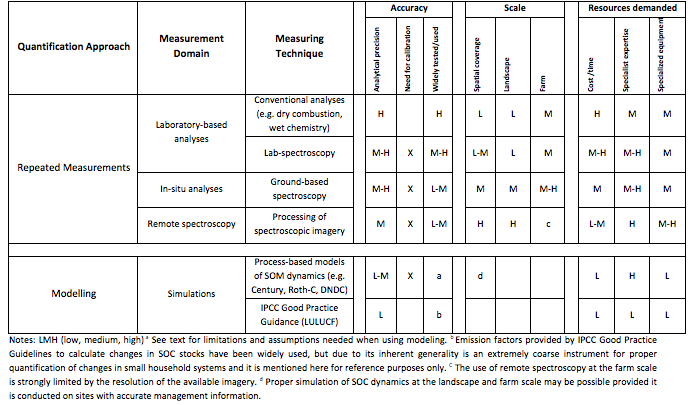
The determination of the sampling intensity required to demonstrate a minimum detectable difference in SOC stocks over time has been the subject of numerous studies (Garten and Wullschleger 1999; Conen et al. 2004; Smith et al. 2004). ). The actual number of samples to detect SOC differences for different degrees of statistical confidence will be directly dependent on the background level that the study requires (i.e. the detectable difference in SOC relative to the stock baseline estimated in the first inventory). Moreover, considering the inherent natural variability of soil properties, the demonstration of small changes in SOC stocks may often require the collection of an impractically large number of samples (Garten and Wullschleger 1999), whose costs may quickly overrun any financial benefit derived from a potential increase in SOC levels. Therefore, different approaches have been used to monitor SOC stock changes, which invariably represent a compromise between accuracy and cost. Table 7.2 shows a comparison of methods used to monitor SOC stock changes classified according to the level of accuracy, scale and resources demanded.

7.3.1 Repeated measurements

A further classification is made on the basis of the measurement domain (where the analyses take place).

Laboratory-based analyses These are the most widely used techniques, which involve physical collection and subsequent processing of soil samples (see section 7.2.3). The standard methods used for soil carbon analysis are dry combustion, wet oxidation, and the use of reflectance spectroscopy, which is increasingly being used over the past number of years as an effective way to optimize time and analytical costs. However, some controversy still exists about the compatibility of data derived from different spectroradiometers (Reeves 2010), and there is still a need for collection and analyses by conventional techniques of a significant proportion of samples to allow for calibration of the entire sample set.

In-situ analyses While lab-based analyses provide high quality results, they are resource-demanding and may be impractical or too expensive for continuous monitoring of SOC (Aynekulu et al. 2011; Batjes 2011). The implementation of SOC analyses in the field by means of portable spectroscopy allows for the assessment of a much larger number of sampling locations compared to that offered by lab-based methods, as the former is a fast, cost-effective and non-destructive technique. However, its accuracy is lower than that provided by conventional methods, since there are issues related to soil surface conditions such as soil moisture and surface roughness, which may affect the spectral signal. Therefore, there is a need to conduct a statistical calibration before each field campaign in order to achieve an acceptable level of accuracy (Stevens et al. 2006).

Table 7.2 Comparison of methods for monitoring SOC stock changes with regard to level of accuracy, scale and resources demanded

Remote spectroscopy The use of reflectance spectroscopy on airborne or satellite-mounted sensors provide high temporal resolution and allow for an improved representation of the spatial variation of SOC in a cost-efficient manner (Ladoni et al. 2010; Croft et al. 2012; Stevens et al. 2006). Nonetheless, there are still major constraints with regard to using this technique as a plausible method to detect SOC stock changes. Croft et al. (2012) highlight some of these limitations, which include: the comparatively higher analytical uncertainty than that obtained from conventional or ground-based reflectance spectroscopy; the high spatiotemporal variability of soil surface conditions that can affect the spectral signal (e.g. soil moisture, vegetation or crop residue cover, differences in soil surface roughness, etc.); the spatial uncertainties associated with instrument spatial resolution and SOC spatial heterogeneity; and the need for atmospheric correction and simultaneous ground data collection to calibrate and validate the output of such studies. Furthermore, remote spectroscopy can only use the reflectance of bare surface to measure soil properties and is not able to detect vertical gradients in SOC within the topsoil (Stevens et al. 2006). Finally, there is a dearth of studies using remote spectroscopy in arid or semi-arid regions, which host a large amount of small household farming systems. In these environments SOC contents are typically low and the interference with other soil properties (e.g. CaCO3 or CaSO4 contents) may change the spectral behaviour of soil considerably, which could have further detrimental effects on the performance of the remote sensing techniques (Ladoni et al. 2010). Withal, the detection limit of these techniques is still too high to use them for SOC stock change studies (Stevens et al. 2006). To make these techniques fully operative, additional efforts must be done to decrease the detection limit.

7.3.2 Modelling

Compared to measuring techniques that require the implementation of repeated measurements to quantify SOC stock changes, the use of process-based models (e.g. DNDC, Roth-C, Century) have obvious advantages in terms of resources demanded. Moreover, models can provide relatively fast and inexpensive simulations of SOM dynamics at different spatiotemporal scales. However, such simulations are based on a number of assumptions that will necessarily result in very large uncertainties of the estimates obtained. Here, we briefly describe some of the main weaknesses of models that could potentially be used to quantify SOC stock changes within the context of small household agricultural systems in tropical environments.

Assumption of stable conditions Most SOM dynamic models assume stable conditions in SOM pools prior to modelling how factors like management or climate change affect their dynamics. However, the vast majority of small household systems in the tropics are not necessarily in steady state conditions. In the tropics, large tracts of land under current agricultural practices have been covered by natural ecosystems not much longer than a generation ago, but in many cases this would only be a few decades or even just some years ago (Houghton 1994; FAO & JRC 2012). Because of this, current SOM dynamics will still be highly influenced by past vegetation. Therefore, the assumption of stable conditions in those systems is likely to result in gross inaccuracies. While the influence of past vegetation might of course be modelled, this would be done at the expense of bringing on further uncertainty to the results, as this impact is likely to vary with type of vegetation, time since conversion, landscape position, soil type, etc.

Coupling erosion processes Quite a significant number of small household systems are established on slopes of varying degrees, with farms being increasingly established on steep marginal land as a result of population pressure. Moreover, cropped fields may be void of vegetation for some time during the year, or in some cases, the entire year (fallow). The combination of those factors makes soil erosion a highly significant factor, which may naturally lead to lateral transfers of SOM. Again, coupling a soil erosion model to a SOM dynamic one can be attempted, but the resultant application would need to be parameterised for the wide array of heterogeneous conditions existing between farm managements, the different land uses, soil types, etc., all of which may undoubtedly produce an even greater source of uncertainty.

Existence of contrasting SOM dynamics between crops Small household systems are highly dynamic in terms of the crops being used (C3 plants such as legumes and napier grass; and C4 plants such maize and sorghum) whose presence and abundance may vary between years within the fields of a given farm. There is increasing evidence that C3 and C4 vegetation have a strong influence on SOM processes, see for instance Wynn and Bird (2007) and more recently Saiz et al. (2015). Besides inherent microbial processes and material (biomass) recalcitrance, these dynamics are highly influenced by soil texture through their effect on abiotic properties. Therefore, vegetation may exert very strong effects on SOC stocks, which traditional SOM dynamic models are not yet able simulate. In summary, models can provide very useful indications about trends of SOM levels with respect to changes in climate and/or management, and they can do so at high spatiotemporal resolutions and at a fraction of the cost of those using repeated measurements (Table 7.2). However, the uncertainties associated to the estimates are currently too large to use them as a verifiable tool to demonstrate SOC stock changes, particularly in these highly heterogeneous systems. At the very least, models require high quality data gathered at different time intervals for proper parameterisation, and this is still an important aspect clearly lacking for these grossly understudied tropical systems (Rosenstock et al., Chapter 9).

7.3.3 Monitoring frequency and recommendations

While IPCC (2003) and IPCC (2006) recommend five-year and 10-20 year monitoring intervals respectively, a relevant sampling interval suited to site-specific conditions can be ascertained by using models of SOC dynamics to plan both the frequency and intensity of subsequent surveys for determining SOC stock changes (Smith 2004). However, modelling of highly heterogeneous environments such small household agricultural systems in tropical systems is a challenging task, which is unlikely to provide a single answer with regard to when and how intensively different sites should be measured to detect significant changes in SOC stocks. Alternatively, estimation of changes in SOC over shorter periods could be achieved through the measurement of changes in particular soil carbon fractions (e.g. particulate organic matter) given that these are more sensitive to changes than total carbon in the bulk soil (Six et al. 2002). While this is a rather useful qualitative assessment of SOC sequestration it does not reflect overall SOC stock changes that should be simultaneously assessed, thus increasing the overall cost and sampling effort. Furthermore, the implementation of a SOM fractionation procedure requires specific laboratory equipment (i.e. sonicator) and access to relatively expensive consumables (i.e. heavy liquid; Wurster et al. 2010).

We recommend adopting a strategy similar to the one proposed by Lark (2009), which suggests sampling only a proportion of the initial baseline sites in any one stratum. This strategy purposely focuses efforts in those locations likely to show the larger differences in SOC stocks over a fixed term (i.e. 10-year period). Thereafter, the strata that show a large change could then be sampled more intensively. Locations likely to show the larger changes in SOC stocks will normally include fields affected by intensive management, those having changed land use since the last survey, and the ones presenting recent signs of land degradation. We also advise pairing sampling locations in space as this may allow for a more effective detection of SOC changes in time (Ellert et al. 2007), and a sampling scheme consistent with that used in the first round of sampling. Furthermore, collection of samples should be routinely conducted at roughly the same time of the year, and in between relevant agricultural practices (i.e. harvesting, fertilization, etc.). Further information about quantifying SOC over time is given in the Appendix A.

We would like to conclude this section on SOC stock changes stressing that the only way to detect reliable signals and early trends in soil monitoring schemes is to improve the overall measurement quality (precision and bias) and to shorten the measurement periodicity (Desaules et al. 2010). However, the labour, analytical costs and time needed to achieve a given sensitivity might overrun the potential monetary benefits derived from a hypothetical increase in SOC levels. As an illustrative case, Smith et al. (2001) indicate that between 10 and 20 samples should be collected to detect a 15% change in SOC stocks in a relatively homogeneous system (<25% coefficient of variation). Moreover, special attention should also be placed on the issue of permanence as most of the new SOC fixed as a result of improved management activities is in a labile form (particulate organic carbon), and thus, it is highly prone to be lost back to the atmosphere in a relatively short timeframe if conditions changed. Therefore, emphasis should be placed on promoting sustainable agricultural practices, as these will bring both economic and environmental benefits to the farmers in the medium term. Enhanced SOC sequestration may indeed be one of those benefits, but in our view it should not be the purpose of grand resource-demanding monitoring schemes, especially if the time elapsed between surveys has not been long enough (i.e. at least 10-20 years). Bearing this in mind, and even considering that at present proper simulation of SOM dynamics is very limited in small household systems because of the scarcity of high quality data, modelling still represents an alternative that, provided high quality data was available, could be applied across broad spatiotemporal scales in a cost-effective manner. Therefore, we propose the establishment of permanent monitoring sites across a gradient of management qualities (from highly intense to poor management scenarios) in the geographical area of interest to serve as reference sites to generate data that can be used for model parameterization and validation for farming practices under small household conditions.

Author affiliations

1 Karlsruhe Institute of Technology, Institute of Meteorology and Climate Research, Atmospheric Environmental Research (IMK-IFU), Kreuzeckbahnstrasse 19, 82467 Garmisch-Partenkirchen, Germany

2 Institute of Research for Development (IRD), Montpellier, France

Appendix A: Methodology for quantification of soil carbon stocks and carbon stock changes

Number of plots required

The number of plots required to estimate SOC stocks in each defined stratum depends on the desired precision, often set at ±10% of the mean at 90 or 95% confidence level. In the case of strata defined by ancillary variables, the number of plots per stratum can be ascertained through the relationship described by Snedecor and Cochran (1967);

where:

t_α is Student’s t with degrees of freedom at either 0.95 or 0.90 probability level, S and D are the standard deviation and the specified error limit respectively for values obtained from an initial assessment of the stratum.

On the other hand, and for the case of a given area stratified by geographical coordinates, the number of samples required could be determined using a slightly modified relationship (Pearson et al., 2005; Aynekulu et al., 2011);

where:

t_α, S and D are as above and derive from values obtained from an initial assessment of the area considered, N is the number of sample units in the population, that is the total area divided by plot size. The resultant number of plots can be further allocated into a number of defined strata by using:

where:

N_h is the area of the stratum h , S_his the standard deviation of stratum h, L is the number of strata, and n are the number of total plots.

In the cases where the confidence interval exceeds +/- 10% with 90% confidence, the user may undertake one of three actions (VCS module VMD0018): a) re-stratify according to any significant correlation observed between the sample variance and geographic or other factors, b) Increase the number of plots, and c) set lower confidence intervals, increasing thus the estimates uncertainty. The determination of the number of plots to be sampled in each stratum as a proportion of both its area and the observed variance may certainly be an efficient approach. Adding to this efficiency, it can also be expected that the number of plots required for determination of SOC stocks for a given stratum defined by ancillary variables may be significantly small compared to the ones needed in the less homogeneous strata defined by geographical coordinates.

With regard to the number of samples required to demonstrate a given minimum detectable difference in SOC stocks over time the reader is referred to Garten and Wullschleger (1999); Conen et al., (2004) and Smith et al., (2004) for sound descriptions of the methods and equations used. Finally, a very recent report by Chappell et al. (2013) provides excellent advice on a generic monitoring design to detect changes in SOC, which includes illustrative examples with step-by-step calculations.

Appendix B: Simplified protocol for taking and processing soil samples, adapted for the SAMPLES Project

This protocol covers both the soil sampling procedure and sampling processing and assumes the plots/subplots to be sampled have already been pre-selected

Soil sampling

Soil samples are collected in four different locations within the plot of choice to account for the inherent heterogeneity of SOC.

Start roughly at the centre of the plot/subplot (replicate 1) and establish the other 3 replicates laid out according to a pattern of three axes separated 120 degrees with respect to an initial axis pointing north. Make sure the other three replicates are set up at a prudent distance from the edges of the plot/subplot (+5 m if possible) to avoid any boundary effects, but do try to cover ground. The final sampling locations will be geo-referenced using a GPS.

It is assumed that a stainless steel corer, a soil auger and/or a spade will be used for retrieving the samples. All samples will be placed in labeled zip-lock bags. It is very important that the bags are clearly labeled with permanent marker. Always a good idea to label them immediately after you take the sample otherwise they may get mixed up (if a marker is not around, write it in a paper and put it inside of each bag). A good labeling should mention at the very least:

• Plot/subplot name or number (e.g. DCR)

• Replicate number (e.g. 3 for replicate 3)

• Depth (i.e. 10-30)

Then in the same bag and line in big clear letters following the example given it should say: DCR-3 (10-30)

Detailed Sampling Procedure

In the case of the 0-10 and 10-30 cm intervals, 3 individual samples within 1 metre radius will be collected. This is done to better account for local heterogeneity, which is particularly pronounced at this shallow depth. Subsequently samples from the same location and depth interval are pooled to minimize analytical costs.

0-10 cm

• Remove vegetation and surface litter.

• Push short corer (steel cylinder) into soil until the 10 cm mark is reached. Retrieve it gently by carefully shaking it back and forth sideways to compact a bit the surrounding soil (this will get subsequent sampling at depth much easier and will avoid soil crumbling into the hole).

• Pull the corer out rotating carefully (always clockwise as this will be very relevant when using the other soil sampling gear at depth)

• Place the soil into plastic bag, trying not to touch it with the hands. Starting with the topside (loose crumbly soil gets out first), and then turn the cylinder upside-down.

• To help the soil come out, use the rubber mallet to impact the cylinder walls while it gets turned around. The soil will come out eventually. Get all the soil out of the tube.

10-30 cm

• Hammer the next sampling cylinder into the soil until the depth markings. You may be using a regular cylinder or the one with a detachable cutting edge (preferably the latter as it is more robust). If using the latter, then you will have to carefully detach this cutter and scrap the sample out onto the bag. This can be done by a second person, thus improving sampling speed. Regardless, beware of what you are using as the diameters (crucial for bulk density determination) change for each choice.

• Shake it back and forth carefully sideways (to compact surrounding soil).

• Rotate clockwise, pull out and extract soil sample (using the sample extruder if using cylinders without detachable cutting edge).

• Again: put the soil into a labeled plastic bag avoiding contact with the hands.

30-50 (55) cm

• If the soil is relatively soft and free of stones, use the cylinders (as bulk density can still be used). If that is not the case, then use the soil auger or spade.

• If you are using the cumulative mass coordinate system to calculate SOC stocks, then you will need to collect all of the soil at the suggested depth intervals plus an extra one a bit deeper (50-55 cm).

• If using a spade to reach the required depth, the sample will be obtained by scratching the soil out of the walls. Prior to obtaining any sample the walls of this hole (pit) need to be cleaned (scratched) to avoid contamination. Start scratching/ sampling from the bottom once the hole has been finished. Take roughly the same amount of soil material along the targeted depth interval, as you do not want to take most of your sample at a concentrated point. It would be good to have a graduated ruler or stick with depth marks.

In general, also consider the following:

• Take notes that may help you to interpret results later on (GPS, land use history, farmers’ comments on management, type of soil, current vegetation, evidence of erosion, fire, etc…).

• If using coring, a sample that comes broken in the first 30 cm (as a result of coarse stones/roots) cannot be used. Sampling has to be done again in another location nearby.

• Beware that if the soil is very rocky, there will be a risk of overestimating SOC stocks if using soil coring. Therefore, an estimate of rock content for a given plot should be given. However, an accurate quantification of rockiness is a very demanding task, as it would involve to purposely sampling several pits at each studied field.

• Always take note of what corer you are using (because of diameters!). It may be that you are exchanging between cylinders with different sizes for whatever logistical reason (e.g. cylinder with detachable cutting hoe vs normal cylinder. These two have different diameters and will definitely affect bulk density calculations). This is very important, take notes.

• Be careful that the sampling hole does not get contaminated while taking samples, e.g. do not step on the hole, do not let litter or surface soil fall in, etc.

• After sampling a plot, the coring cylinders and scraper need to be thoroughly cleaned (have wet cloths with you).

• If using the auger, use the same depth intervals as those with the cores (0,10, 30, 50).

• From the outside of the plastic bag, crumble by hand big clumps of soil into smaller parts, which will be critical for easy soil processing later on.

• Closure of bags: rolling them up releasing air from the bag and then close it, so that it contains as little air as possible.

• Take several pictures of the plot/subplot.

• As a matter of good practice, do try to fill in sampling holes with any excess soil derived from your digging.

• To calculate SBD using the auger, you will need to calculate the volume by filling the hole with sand, which is highly demanding and slow procedure.

Soil bulk density (SBD) determinations

In all cases, calculation of SBD should include fractions >2 mm. So before any sieving takes place the following should be done:

As soon as possible, and certainly before 2 days after collection from the field, let the samples air-dry (after opening and rolling down bags) in a rain-protected location. It is always a good idea to progressively (each day) break the soil clumps with your fingers while the bags are being dried (but be gentle or you may break the bag). A bit everyday is the best, otherwise you will find handling of samples much harder in the coming days, and will have to use a hammer. Also, avoid cross-contamination between samples by doing it from the outside of the bag (gently squeezing it with your fingers). When an oven becomes available, put the bags inside at 40 °C. After a number of days, when samples are seemingly dry (5-7 days will be safe- but of course it all depends on initial moisture content), take them out of the oven and weigh each sample (including the plastic bag) but wait about half an hour after the samples have been taken out to do this weighing.

After this weighing, take an aliquot of each sample and place them in labeled paper bags (about ~ ¼, of the total sample, but weigh how much exactly before you put them inside the oven). Dry them at 105 °C for 24 h. As before, weigh all the samples after about half an hour after they were taken out of the 105 degrees oven. Once the weights of these aliquots have been recorded you can throw this material away.

In total you should have 3 weighs for each sample (i.e. total soil weight, sample before oven dried at 105°C, sample after oven dried at 105°C). This will allow for proper calculation of soil bulk density (SBD).

In general, also consider the following:

• Make sure you always take weights knowing which bag you are using as each different type of bag will have different weight (both plastic and paper).

• Get an average weight of 5 bags of each type you use, so that can be deducted from the calculations later on.

• Let the samples dry by air (open plastic bag) and roll them down

• Always check that the oven works well.

• Let the samples cool down at room temperature for at least 30 min, unless there was a desiccator that could be used for storing samples prior to weighing. In such case, then the weighing should occur immediately after extracting the samples from the desiccator.

• Weigh the soil with its bag. Very Important!

• Balance/scale should be precise up to 0.1g.

Sample processing

Sieving: The remaining of each sample dried at 40 degrees (most of it) needs to be weighed again and sieved to 2 mm. Gravel and root content >2 mm will be weighed separately. Therefore we will get the fractions of coarse roots and gravel. But first remove carefully all large clumps with a rolling pin (bakery). Removing the soil from the bag to break up any clumps is very time consuming and may lead to gross errors. Therefore, it is good practice to progressively break clumps from the outside of the bag as the sample dries. After sieving, you should have 3 weighs for each sample (bag) in total (i.e. total soil weight, roots>2 mm, and gravel (>2 mm)).

Pooling/bulking: There are numerous ways of pooling, and the final choice depends on the purpose and load of work that can be undertaken. The methods explained below are just two ways that lead to fewer analyses to be undertaken and cover two different purposes:

1. If the aim is to get bulk soil samples to undertake just a single analyses at each plot/subplot bulk by depth interval (e.g. all samples from the same plot/subplot collected at 10-30 cm), then do as follows:

• Use the same weigh for all the replicates (20 or 30 g), and put them together in a bowl or tray. Do not use the entire sample from each bag! Keep them as back ups.

• Mix them a bit always with clean, dry hands (10 sec should be alright).

• Put the mixture in a new bag with the same code as before but indicating ‘Bulk” at the end.

• If the aim is to also get a ‘master soil sample’ 0-30 cm for subsequent analyses (texture, mineralogy, organic matter fractionation, ECEC, etc.) then from the previous bulked bags the weights that need to be put together are calculated as follows:

• First the average bulk density for the Master (BDM) is calculated:

BDM= [BD(0-10) x (1/3)] + [BD(10-30) x (2/3)]

• Then to obtain about 90 g of Master sample, proceed as follows:

30 g x BD(0-10) / BDM

60 g x BD(10-30) / BDM

• These weights are put in a separate bag, which is to be called ‘master’ with same code as before and indicating (0-30) at the end of the labeling.

2. Sometimes it may be necessary to have an extra bag with about 20 g of Master soil (0-30) that will be used for soil textural analyses. Take about 20 g from this bag and put them into a small bag with the same coding indicating that is for ‘texture’.

Powdering: If powdering is needed, then proceed as follows:

• Take about 3 g of your sieved, pooled/bulked sample.

• Powder the sample with the aid of a mortar-pestle or micro-mill device.

• Put the sample into a small plastic bag with the code on it.

• Be very careful that all instruments used for powdering get properly cleaned (if using water then it is very important that everything is absolutely dry again – or subsequent analyses involving weighing of the sample will be biased).

• Finally, about 50 g of sample per bag should be stored for any further potential analyses.

References

Allen DE, Pringle MJ, Page KL and Dalal RC (2010) A review of sampling designs for the measurement of soil organic carbon in Australian grazing lands. The Rangeland Journal 32: 227-246.

Aynekulu E, Vagen T-G, Shephard K, Winowiecki L (2011) A protocol for modeling, measurement and monitoring soil carbon stocks in agricultural landscapes. Version 1.1. World Agroforestry Centre, Nairobi. http://www.worldagroforestry.org/downloads/publications/PDFs/TM11192.PDF. Accessed January 27, 2015.

Batjes NH (2011) Research needs for monitoring, reporting and verifying soil carbon benefits in sustainable land management and GHG mitigation projects. In: De Brogniez D, Mayaux P and Montanarella L (ed) Monitoring, reporting and verification systems for carbon in soils and vegetation in African, Caribbean and Pacific countries. European Commission, Joint Research Center, Brussels, p 27-39.

Bell MJ, Worrall F (2009) Estimating a region’s soil organic carbon baseline: the undervalued role of land-management. Geoderma 152: 74-84.

Berry N, Cross A, Hagdorn M, Ryan C (2012) The Small-Holder Agriculture Monitoring and Baseline Assessment (SHAMBA). Tropical land use research group. School of GeoSciences. University of Edinburgh. Scotland (UK).

Berry N (2011) Whole farm carbon accounting by smallholders, lessons from Plan Vivo Projects. Presentation at the ‘Smallholder Mitigation: Whole Farm and Landscape Accounting’ Workshop, FAO, Rome, 27-28th October, 2011.

Bird MI, Veenendaal EM, Lloyd J (2004) Soil carbon inventories and d13C along a moisture gradient in Botswana. Global Change Biology 10: 342–349.

Carsky RJ, Jagtap S, Tain G, Sanginga N, Vanlauwe B (1998) Maintenance of soil organic matter and N supply in the moist savanna zone of West Africa. In: Lal R (ed) Soil Quality and Agricultural Sustainability. Ann Arbor Press, Chelsea, Michigan, p 223-236.

Chappell A, Baldock J, Rossel RV (2013) Sampling soil organic carbon to detect change over time. Report to Grains Research and Development Corp. and Australian Department of Environment, Australia.

Conen F, Zerva A, Arrouays D et al. (2004) The carbon balance of forest soils: detectability of changes in soil carbon stocks in temperate and boreal forests. In: Griffith H, Jarvis PG (ed) The Carbon Balance of Forest Biomes. Bios Scientific Press, London.

Croft H, Kuhn NJ, Anderson K (2012) On the use of remote sensing techniques for monitoring spatio-temporal soil organic carbon dynamics in agricultural systems. Catena 94: 64–74.

de Gruijter JJ, Brus DJ, Bierkens MFP, Knotters M (2006) ‘Sampling for Natural Resource Monitoring’. Springer, New York.

Desaules A, Ammann S, Schwab P (2010) Advances in long‐term soil‐pollution monitoring of Switzerland. J of Plant Nutr Soil Sci 173: 525–535.

Ellert BH, Bettany JR (1995) Calculation of organic matter and nutrients stored in soils under contrasting management regimes. Can J Soil Sci 75: 529–538.

Ellert BH, Janzen HH, VandenBygaart AJ, Bremer E (2007) Measuring change in soil organic carbon storage. In: Carter MR, Gregorich EG (Eds.) Soil sampling and methods of analysis, 2nd ed, p 25-38. CRC Press, Boca Raton, FL.

FAO, JRC (2012) Global forest land-use change 1990–2005. E.J. Lindquist EJ, D’Annunzio R, Gerrand A, MacDicken K, Achard F, Beuchle R, Brink A, Eva HD, Mayaux P, San-Miguel-Ayanz J, Stibig H-J. FAO Forestry Paper No. 169. Food and Agriculture Organization of the United Nations and European Commission Joint Research Centre. FAO, Rome.

Garten CT, Wullschleger SD (1999) Soil carbon inventories under a bioenergy crop (Switchgrass): measurement limitations. Journal of Environmental Quality 28: 1359–1365.

Gifford RM and Roderick ML (2003) Soil carbon stocks and bulk density: spatial or cumulative mass coordinates as a basis of expression? Global Change Biology 9: 1507-1514.

Goidts E, Van Wesemael B, Crucifix M (2009) Magnitude and sources of uncertainties in soil organic carbon (SOC) stock assessments at various scales. Eur J Soil Sci 60: 723–739.

GOFC-GOLD (2009) A sourcebook of methods and procedures for monitoring and reporting anthropogenic gas emissions and removals caused by deforestation, gains and losses of carbon stocks in forests remaining forests, and forestation. In: GOFC-GOLD Report version COP15-1. Alberta, Canada, p 197.

Guo LB and Gifford RM (2002) Soil carbon stocks and land use change: a meta analysis. Global Change Biology 8: 345-360.

Hairiah K, Dewi S, Agus F, Velarde S, Ekadinata A, Rahayu S and van Noordwijk M (2010) Measuring Carbon Stocks Across Land Use Systems: A Manual. World Agroforestry Centre (ICRAF), SEA Regional Office, Bogor, Indonesia.

Houghton RA (1994) The worldwide extent of land-use change. BioScience 44(5): 305–313.

IPCC. Agriculture, in Climate Change (2007): Mitigation. Working Group III Contribution to the Fourth Assessment Report of the Intergovernmental Panel on Climate Change. Cambridge University Press, New York

IPCC (2003) Good Practice Guidance for Land Use, Land-Use Change and Forestry. Penman J, Gytarsky M, Hiraishi T, Krug T, Kruger D, Pipatti R, Buendia L, Miwa K, Ngara T, Tanabe K, Wagner F. (Eds.)

IPCC (2006) 2006 IPCC Guidelines for National Greenhouse Gas Inventories Volume 4, Agriculture, Forestry and Other Land Use. Eggleston S, Buendia L, Miwa K, Ngara T, Tanabe K (Eds.)

Ladoni M, Bahrami HA, Alavipanah SK, Norouzi AA (2010) Estimating soil organic carbon from soil reflectance: a review. Precis Agric 11: 82-99.

Lark RM (2009). Estimating the regional mean status and change of soil properties: two distinct objectives for soil survey. European Journal of Soil Science 60: 748–756.

Lee J, Hopmans JW, Rolston DE, Baer SG, Six J (2009) Determining soil carbon stock changes: Simple bulk density corrections fail. Agr Ecosyst Environ 134: 251–256.

Lipper L, Neves B, Wilkes A, Tennigkeit T, Gerber P, Henderson B, Branca G, and Mann W (2011). Climate change mitigation finance for smallholder agriculture. In: A guide book to harvesting soil carbon sequestration benefits. Food and Agriculture Organization of the United Nations (FAO) report. FAO, Rome.

McBratney AB, Minasny B (2010) Comment on “Determining soil carbon stock changes: Simple bulk density corrections fail” [Agric Ecosyst Environ 134 (2009) 251–256]. Agric Ecosyst Environ 136: 185–186.

MacDicken KG (1997) A Guide to Monitoring Carbon Storage in Forestry and Agro-forestry Projects. Winrock Internationl Institute for Agricultural Development, Arlington, USA.

McKenzie N, Ryan P, Fogarty P, Wood J (2000) Sampling, measurement and analytical protocols for carbon estimation in soil, litter and coarse woody debris. In: National Carbon Accounting System Technical Report No. 14, Australian Greenhouse Office, Canberra, Australia.

Milne E, Neufeldt H, Smalligan M, Rosenstock T, Bernoux M, Bird N, Casarim F, Deneuf K, Easter M, Malin D, Ogle S, Ostwald M, Paustian K, Pearson T, Steglich E (2012) Overview Paper: Methods for the quantification of net emissions at the landscape level for developing countries in smallholder contexts. CCAFS Report No. 9. CGIAR Reseach Program on Climate Change, Agriculture and Food Security, Copenhagen Denmark.

Milne E, Neufeldt H, Rosenstock T, Smalligan M Cerri CE, Malin D, Easter M, Bernoux M, Ogle S, Casarim F (2013) Methods for the quantification of GHG emissions at the landscape level for developing countries in smallholder contexts Environ Res Lett 8 015019.

Murphy B, Badgery W, Simmons A, Rawson A, Warden E, and Andersson K (2013) Soil testing protocols at the paddock scale for contracts and audits – Market-based instrument for soil carbon. New South Wales Department of Primary Industries, Australia.

Pearson TRH, Brown S, Ravindranath NH (2005) Integrating Carbon Benefit Estimates into GEF Projects. United Nations Development Programme, Global Environment Facility.

Prudencio CY (1993) Ring management of soils and crops in the West African semi-arid tropics: the case of the mossi farming system in Burkina Faso. Agriculture, Ecosystem and Environment 47: 237-264.

Ravindranath, NH and Ostwald M (2008) Carbon Inventory Methods: Handbook for Greenhouse Gas Inventory, Carbon Mitigation and Roundwood Production Projects. Advances in Global Change Research 29. Springer, New York, NY

Reeves JB (2010) Near-versus mid-infrared diffuse reflectance spectroscopy for soil analysis emphasizing carbon and laboratory versus on-site analysis: where are we and what needs to be done? Geoderma 158: 3-14

Rosenstock TS, Rufino MC, Chirinda N, Bussel L, Reidsma P, Butterbach-Bahl K. Scaling point/plot measurements of greenhouse gas fluxes, balances and intensities to whole-farms and landscapes. This volume.

Saiz G, Bird M, Domingues T, Schrodt F, Schwarz M, Feldpausch T, Veenendaal E, Djagbletey G, Hien F, Compaore H, Diallo A, Lloyd J (2012) Variation in soil carbon stocks and their determinants across a precipitation gradient in West Africa. Global Change Biology 18: 1670-1683.

Saiz G, Bird M, Wurster C, Quesada CA, Ascough P, Domingues T, Schrodt F, Schwarz M, Feldpausch TR, Veenendaal E, Djagbletey G, Jacobsen G, Hien F, Compaore H, Diallo A, Lloyd J (2015) The influence of C3 and C4 vegetation on soil organic matter dynamics in contrasting semi-natural tropical ecosystems. Biogeosciences 12: 5041-5059.

Shepherd KD, Walsh MG (2002) Development of reflectance libraries for characterization of soil properties. Soil Sci. Soc. Am. J. 66: 988-98.

Shepherd KD, Walsh MG (2007) Infrared spectroscopy—enabling an evidence-based diagnostic surveillance approach to agricultural and environmental management in developing countries. Journal of Near Infrared Spectroscopy 15: 1-19.

Singh K, Murphy BW, Marchant BP (2013) Towards cost-effective estimation of soil carbon stocks at the field scale. Soil Research 50: 672-684.

Six J, Callewaert S, Lenders S et al. (2002) Measuring and understanding carbon storage in afforested soils by physical fractionation. Soil Science Society of America Journal 66: 1981–1987.

Smith P, Falloon P, Smith JU et al (ed) (2001) Soil Organic Matter Network (SOMNET): 2001 Model and Experimental Metadata. GCTE Report 7, 2nd edn. GCTE Focus 3 Office, Wallingford, Oxon.

Smith P (2004) How long before a change in soil organic carbon can be detected?” Global Change Biology 10(11): 1878-1883.

Snedecor GW, Cochran WG (1967) Statistical methods. Iowa State University Press, Ames, Iowa, USA p 274.

Stevens A, Van Wesemael B, Vandenschrick G, Touré S, Tychon B (2006) Detection of carbon stock change in agricultural soils using spectroscopic techniques. Soil Sci Soc Am J 70: 844–850.

Subedi BP, Pandey SS, Pandey A, Rana EB, Bhattarai S, Banskota TR, Charmakar S, Tamrakar R (2010). Guidelines for measuring carbon stocks in community managed forests. Asia Network for Sustainable Agriculture and Bioresources (ANSAB), Federation of Community Forest Users, Nepal (FECOFUN), International Centre for Integrated Mountain Development (ICIMOD) Norwegian Agency for Development Cooperation (NORAD).

Tittonell P, Vanlauwe B, Leffelaar PA, Rowe E, Giller KE (2005a) Exploring diversity in soil fertility management of smallholder farms in western Kenya. I. Heterogeneity at region and farm scale. Agric. Ecosyst. Environ. 110: 149–165

Tittonell P, Vanlauwe B, Leffelaar PA, Shepherd KD, Giller KE (2005b) Exploring diversity in soil fertility management of smallholder farms in western Kenya. II. Within-farm variability in resource allocation, nutrient flows and soil fertility status. Agric. Ecosyst. Environ. 110: 166-184.

Tittonell P, Muriuki A, Klapwijk CJ, Shepherd KD, Coe R, Vanlauwe B (2013) Soil heterogeneity and soil fertility gradients in smallholder farms of the East African Highlands. Soil Science Society of America Journal 77: 525-538.

Vågen T-G, Winowiecki LA, Tamene Desta L, Tondoh JE (2015) The Land Degradation Surveillance Framework (LDSF) – Field Guide v4.1. World Agroforestry Centre, Nairobi, Kenya, 14 pp.

Veldkamp A, Kok K, de Koning GHJ, Verburg PH, Priess J, Bergsma AR (2001) The need for multi-scale approaches in spatial specific land use change modelling. Environmental Modeling and Assessment 6: 111–121.

Verified Carbon Standard (2012) VCS Module VMD0021: Estimation of Stocks in the Soil Carbon Pool. VCS, Washington DC, USA.

Wuest SB (2009) Correction of bulk density and sampling method biases using soil mass per unit area. Soil Sci. Soc. Am. J. 73: 312–6.

Wurster, CM, Saiz G, Calder A, Bird MI (2010) Recovery of organic matter from mineral-rich sediment and soils for stable isotope analyses using static dense media. Rapid Commun. Mass Spectrom. 24: 165–168.