Todd S. Rosenstock¹, Mariana C. Rufino², Ngonidzashe Chirinda, Lenny van Bussel, Pytrik Reidsma, Klaus Butterbach-Bahl6,7
Abstract: Measurements of nutrient stocks and greenhouse gas (GHG) fluxes are typically collected at very local scales (< 1 to 30 m2) and then extrapolated to estimate impacts at larger spatial extents (farms, landscapes, or even countries). Translating point measurements to higher levels of aggregation is called scaling. Scaling fundamentally involves conversion of data through integration or interpolation and/or simplifying or nesting models. Model and data manipulation techniques to scale estimates are referred to as scaling methods. In this chapter, we first discuss the necessity and underlying premise of scaling and scaling methods. Almost all cases of agricultural GHG emissions and carbon (C) stock change research rely on disaggregated data, either spatially or by farming activity, as a fundamental input of scaling. Therefore, we then assess the utility of using empirical and process-based models with disaggregated data, specifically concentrating on the opportunities and challenges for their application to diverse smallholder farming systems in tropical regions. We describe key advancements needed to improve the confidence in results from these scaling methods in the future.
Table of contents:
9.1 Why estimate GHG impacts at whole-farm and landscape level?
9.2 Scaling methods
9.3 Using empirical and process-based models with disaggregated data
9.4 Conclusion
Author affiliations
References
9.1 Why estimate GHG impacts at whole-farm and landscape level?
Agricultural systems are a major source of atmospheric greenhouse gas (GHG) emissions, contributing approximately 30% to total anthropogenic emissions if land use change is included (Vermeulen et al. 2012). To better target interventions aimed at reducing GHG emissions from agricultural systems, there is a need for information on GHG balances and the GHG intensity of agricultural products (e.g., emissions per unit product) at levels where livelihood and environmental impacts occur and land management decisions are being made. However, even in smallholder farming systems where decisions are taken on fields and farms that are usually less than one hectare, this decision scale is substantially greater than the scale at which changes in GHG fluxes take place or are measured, often that of micrometers and meters (Butterbach-Bahl et al. 2013). The factors regulating nitrous oxide (N2O) generation in agricultural fields illustrate this point. At the scale of soil aggregates—mm in size–soil moisture affects oxygen available to microbes, driving denitrification (the conversion of NO3O to N2O principally by facultative anaerobic bacteria). Meanwhile, soil moisture, influenced by the percentage of water filled pore space, is regulated by precipitation and soil tillage—events determined at a larger spatial extent. Furthermore, heterogeneous distribution of decomposing residues from the previous harvest may lead to formation of denitrification and N2O hotspots at the cm scale, thereby triggering changes in the magnitude and spatial variability of fluxes even at plot scale (Groffman et al. 2009). Consequently, land-based mitigation actions require a lower resolution of information than that needed to explain the processes driving GHG emissions at the soil-plant-atmosphere interface.
GHG fluxes are typically measured at locations or ‘points’, intended to be representative of a larger area. Independent of source, sink or molecule, GHG measurements – for example chamber measurements of fluxes O are conducted on only a fraction of the area or a few of the landscape units because of costs and complexity (Rufino et al. 2016; Butterbach-Bahl et al. this volume). When attempting to understand landscape or regional GHG fluxes or consider mitigation options, it is therefore necessary that these point measurements be translated to larger extents where effective and meaningful mitigation actions can be taken.
‘Scaling’ GHG flux measurements underlies GHG accounting (e.g., national inventories), and forms the basis for policy analysis (e.g., marginal abatement cost curves), development strategies (e.g., low emission development), and even simple testing of mitigation options (e.g., comparing impacts of one practice versus an alternative). Thus, it is important to understand basic principles and terminology that pertain to scales and scaling, to avoid confusion in discussions and analysis. Scale refers to the spatial or temporal dimension of a phenomenon (van Delden et al. 2011; Ewert 2004). Scaling refers to the transfer of information between scales or organizational levels (Blöschl and Sivapalan 1995). Scaling methods refer to tools required to accomplish scaling. This chapter is concerned with understanding the theory and practice behind scaling methods as applied to GHG measurements and impacts.
9.2 Scaling methods
Most scaling methods are grounded in ecological hierarchy theory. Hierarchy theory provides a conceptual framing for scaling in that it structures systems as nested levels of organization (Holling 1992). Components are arranged within higher levels; for example, a field is part of a farm that can be thought of as part of a landscape; moreover, these different components are spatially heterogeneous areas of interacting patches of ecosystems (Fig. 9.1). Scaling methods rely on this conceptual framing to infer relationships between attributes and to translate values derived from point measurements into estimates across scales.
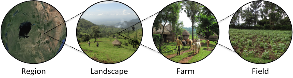
Table 9.1 Conceptual framework of select scaling methods. Based on Ewert et al. (2011)
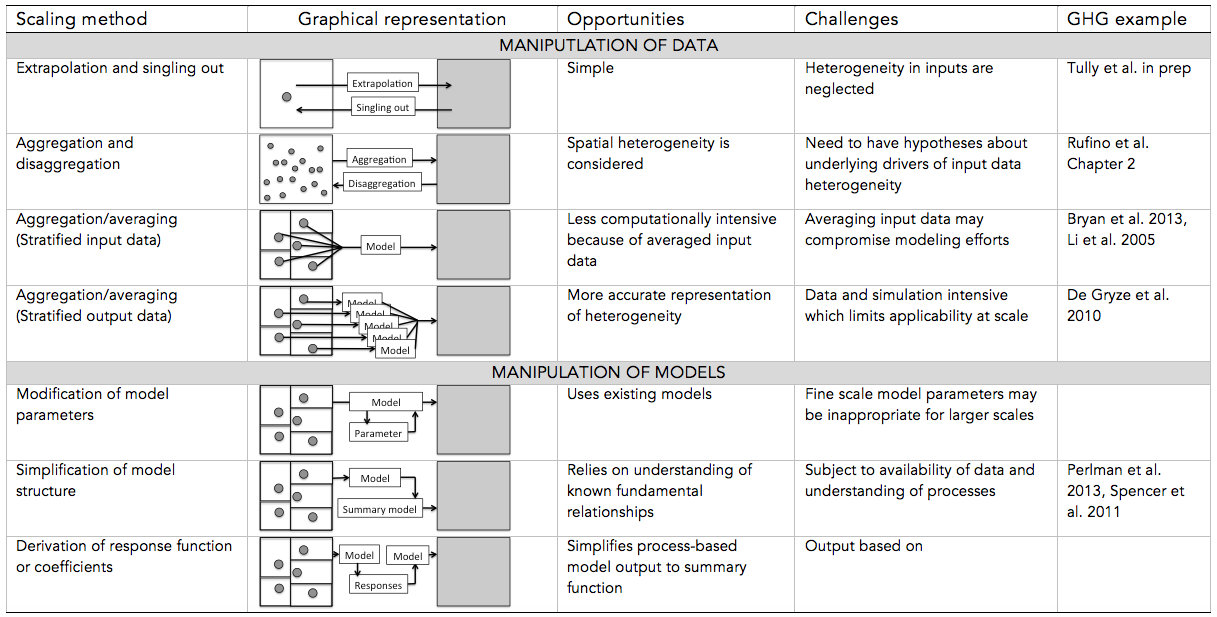
Scaling methods can be categorized into two groups: (1) manipulation of input or output data or (2) manipulation of models (Volk & Ewert, 2011). Approaches that manipulate data are extrapolation, interpolation, (dis)aggregation, or averaging sampled input data (i.e., point measurements) to generate estimates at larger scales (Table 9.1). National Greenhouse Gas Inventories that use IPCC default Tier 1 emission factors (IPCC 2006) are an example of a scaling method that uses a data manipulation approach, namely disaggregation and aggregation. Agriculture is disaggregated into farming activities and their extents (e.g., size of cattle population or tons of nitrogen (N) fertilizer applied) for which a coefficient or empirical model derived from point measurements of the relationship between that activity and GHG fluxes (i.e., empirical model) is then used to calculate emissions at national or sub-national levels. Data manipulation approaches are among the simplest approaches to implement, especially in regions and for production conditions where data are sparse. However, since data manipulation approaches generally neglect heterogeneity in GHG emissions and underlying physicochemical and biological processes, estimates may not represent observed fluxes well at the site level. However, in most cases for developing countries, the accuracy of using such methods is unknown because there are insufficient data to evaluate the variation of source events (input data) or the accuracy of outputs. The ability to generate accurate estimates at larger temporal or spatial scales by manipulating data depends on (1) representative sampling of the disaggregated GHG source/sink activities and (2) the availability of a reasonable model— empirical or process-based—to scale input data. Recently, novel approaches for disaggregation of national, landscape or farm components such as stratification by socio-ecological niches using a combination of household surveys and remote sensing and stratification by agroecological conditions using existing climate, soils and management information have been evaluated to improve estimates because of the better representation of the heterogeneity found in plots, fields, farms and landscapes (Hickman et al. 2014; Rufino et al. 2016).
The alternative to manipulating data is to modify existing models to be relevant at larger spatial scales. This has been successfully done for national-scale soil C monitoring in the US, where an integrated data collection and biogeochemical process-based model (DAYCENT) estimates changes in soil C stocks (Spencer et al. 2011). However, other examples for agricultural GHG impact assessments remain scientific exercises (see Perlman et al. 2013 for national scale N2O assessment). Approaches to manipulate models change model structure to account for the availability and resolution of input data and to make them computationally tractable. Reformulation of model structure (not creating of new models) can result in a reduction of parameters (e.g., macroecological models of functional traits) or simplified model functional forms (e.g., empirical equations derived from multiple runs of process-based models). An important consideration is that scaling by modifying models introduces uncertainty: uncertainty in the quality and quantity of input data, uncertainty of datasets used to test models, and uncertainty related to model structure and parameters in the revised models.
Theory supporting the manipulation of data and models as well as potential errors/uncertainties in outcomes is reviewed in the integrated assessment literature (e.g. Ewert et al. 2011; Volk and Ewert 2011). The process of selecting representative sampling points by various stratification methods (e.g., spatially, land cover, farming activity, etc.) are covered in Chapter 2 and measurements techniques for various fluxes and productivity are covered in Chapters 3-8. Here we discuss the two methods most commonly used to scale up point measurements of disaggregation/aggregation data: empirical and process-based models.
Empirical models are usually relatively simple statistical functions constructed based on the relationship between occurrence of activities or external events, farming or rainfall for example, and monitored responses in the magnitude and temporal and spatial variability of GHG fluxes. By contrast, process-based ecosystem models are built upon our current theoretical understanding of the physicochemical and biological processes underlying GHG emissions. They represent current understanding of complex processes and the interactions of C, N and water cycling at the ecosystem scale to simulate the mechanisms that control GHG fluxes. However, process models need detailed input information and have numerous parameters describing key ecosystem processes and some of the algorithms are still empirical and represent apparent flux responses rather than the underlying processes. Unlike empirical models that require calibration each time they are used, one assumes that the simulated processes are universal and, thus, that based on a number of site tests, they might be applied at sites with a different agro-ecological regime for which they have not previously been calibrated, although calibration of specific parameters might still be required. In the following, we briefly describe these two approaches, their applicability for smallholder systems, representation of the landscape units, technical demands of the process and sources of uncertainty.
9.3 Using empirical and process-based models with disaggregated data
9.3.1 Empirical models
Empirical models for scaling GHGs are based on statistical functions that relate land management ‘activities’ such as extent of a land cover type, amount of fertilizer applied, or the number of heads of livestock to changes in GHG emissions or C sequestration. Carbon stock changes, and GHG fluxes can then be calculated based on two types of input data: (1) that describes the occurrence of activities (so called ‘activity data’) and (2) the average effect that an activity has on a nutrient stock or flux in question (‘emission factors’) (equation 9.1).
![]()
where:
GHG equals the stock (mass) or flux (rate: mass per unit time), sequestration or balance in units of C, N or an integration of the two (CO2 eq) A represents the extent (area) over which an activity occurs EF is an emissions factor (e.g., a constant rate relative to the specific activity: mass per unit time per unit area).
Summation of GHG fluxes or stock changes across N activities (sources/sinks) generates a cumulative balance for the selected area. This approach is analogous to a linear aggregation scaling method based on measurements or estimated values.
The most widely applied empirical models for scaling GHGs are contained within the IPCC Guidelines for Greenhouse Gas Accounting (IPCC 2006). The IPCC Guidelines define global (Tier 1) and, sometimes regional (Tier 2) emission factors for GHG sources and sinks such as the methane produced by enteric fermentation per head of cattle or the amount of nitrous oxide resulting from the application of nitrogenous fertilizers. Persons interested in GHG quantification can multiply these values and use the provided equations with locally relevant data on farm and landscape management activities to generate estimates of individual sources and sinks or cumulative GHG balances. Application of emission factors and empirical models is the foundation of national greenhouse gas inventories and data (Tubiello et al. 2013) and is becoming more common for landscape GHG accounting including ex)ante climate change mitigation project impact assessments (Colomb and Bockel 2013).
IPCC Tier 1 default emission factors are based on both empirical data and expert opinion. In some cases, emissions factors are derived from analysis of 100s or even 1 000s of measurements of the source activity and the rates of emissions. For instance, IPCC default emissions factor for nitrous oxide emissions from N fertilizer use (%) are based on the database of nearly 2 000 individual measurements from studies conducted around the world (De Klein et al. 2006; Stehfest and Bouwman, 2006). Distribution of the studies they are taken from is however biased toward measurement campaigns conducted in Europe and North America. Other emission factors are estimated based on very limited data (e.g. single values for carbon stocks in agroforestry systems) or expert opinion (e.g. emission factor for methane emission from enteric fermentation is based on modeled results, not measurements, for Africa) (IPCC 2006). Global default emissions factors are published in the National Guidelines for Inventories while other regionally relevant emissions factors are available in the IPCC Emissions Factor database, peer reviewed literature and in the future will be made available through the SAMPLES web platform.
Empirical models are typically thought to generate reasonable approximations of GHG fluxes at higher levels of organizations and large spatial extent (Del Grosso et al. 2008), presuming the activity data are well constrained. This is because it is thought that at large scales such as across countries, the departure of actual fluxes from average emissions factor values will average out with aggregation of multiple land units. However, for any local scale—farms for example, where local environmental and management heterogeneity of conditions are not well represented in the global datasets, applying empirical models and emissions factors may represent a significant departure from actual fluxes.
The relevance of using empirical models for farmbscale estimates of GHG balances is untested and perhaps spurious, especially for farming systems in developing countries. IPCC guidelines using Tier 1 default factors were not designed for this purpose. Tier 1 approaches were intended to be used when the source activity was relatively inconsequential to total GHG budgets, perhaps contributing less than 5% of the total (IPCC 2006). Furthermore, significant variations in GHG flux rates occur between point locations due to edaphic mechanisms that control biological emission processes. Because observations of GHG fluxes for tropical smallholder farming systems are scarce or nearly missing in available databases, Tier 1 default factors may considerably misrepresent flux rates for such systems. In view of the low use of N fertilizers in sub-Saharan Africa it is therefore not surprising that many of the N2O fluxes currently being measured there are 1/3 to 1/2 of those estimated using the Tier 1 IPCC emission factors (Hickman et al. 2014; Shcherbak et al. 2014). A comprehensive evaluation of Tier 1 emission factors relating to GHG impacts measured in tropical regions is currently lacking. these concerns and the uncertainty of the results, disaggregation of whole-farms into component activities and applying available empirical models remains a way to estimate relative impacts of smallholder farming activities at the whole-farm level (Seebauer 2014), as well as understand emission hotspots and the research gaps.
Emissions from livestock production in the tropics, namely from enteric fermentation and manure management, present their own challenges due to data scarcity (Goopy et al. this volume). Similarly to soil fluxes, emissions from both sources are poorly constrained and according to the review by Owen and Silver (2015) data for dairy manure management are limited in Africa and extremely scarce for other systems (Predotova et al. 2010). Yet in many countries, these sources are thought to be substantial contributors to total GHG budgets (Gerber et al. 2013).
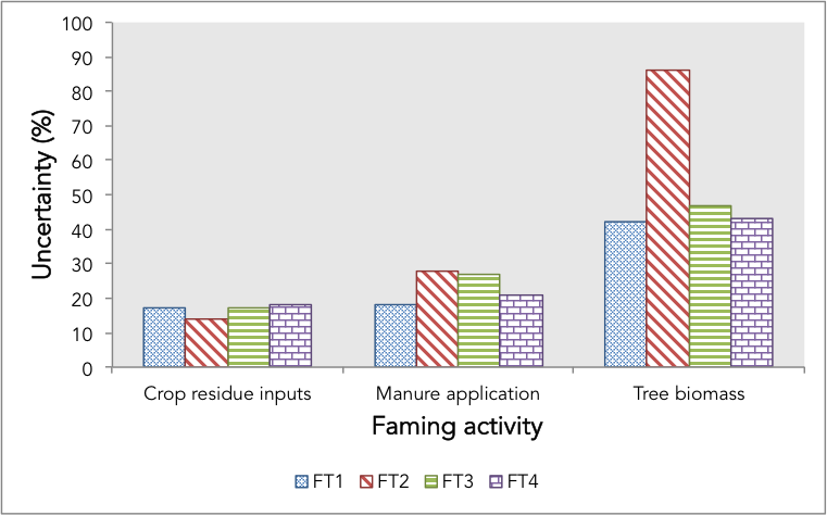
Besides poorly constrained emissions factors, an additional issue (and arguably most important) is limited knowledge of farm management practices (A in equation 1), which limits the use of empirical relationships and models to calculate fluxes. Many developing countries have poorly defined record keeping and reporting schemes about organic and inorganic fertilizer use, manure management, crop rotations and other activities, so there is limited information on the extent of land management decisions (Ogle et al. 2013). This adds another source of uncertainty (in addition to emission factors themselves). Valentini et al. (2014) reported that estimates of the extent of various land cover types in Africa can be from 2.5% to 110% different, depending on the data source, either using inventory sources or satellite imagery (Valentini et al. 2014). Other evidence from data collection methods suggests that the uncertainty in farm management practices is similar to that of emissions, 30 to 80% (Fig. 9.3, Seebauer 2014). New practices have been developed to help developing countries better represent the activities in their agricultural landscapes (Tubiello et al. 2013) and many institutions such as the US Environmental Protection Agency train government personnel in developing countries to cob compile inventories. However, problem with the data quality itself remains. Incentives to improve and standardize data collection and archiving efforts are limited.
Simplicity and transparency are the largest benefits of using data (dis)aggregation techniques and empirical models for scaling GHG estimates. The models represent relationships that are easy to understand and implement, which makes them accessible to next users without requiring much technical expertise. This has led to the creation of a wide range of GHG calculators such as the Cool Farm Tool and EX-ACT (see Colomb and Bockel 2013 for a review). These tools make it possible for nonbspecialist to perform calculations and generate estimates of greenhouse gas balances with relatively little data or effort. It is still unknown, however, whether the estimates produced by such tools provide robust values — either in terms of absolute or relative changes between different practices (Fig. 9.2).
9.3.2 Process-based models
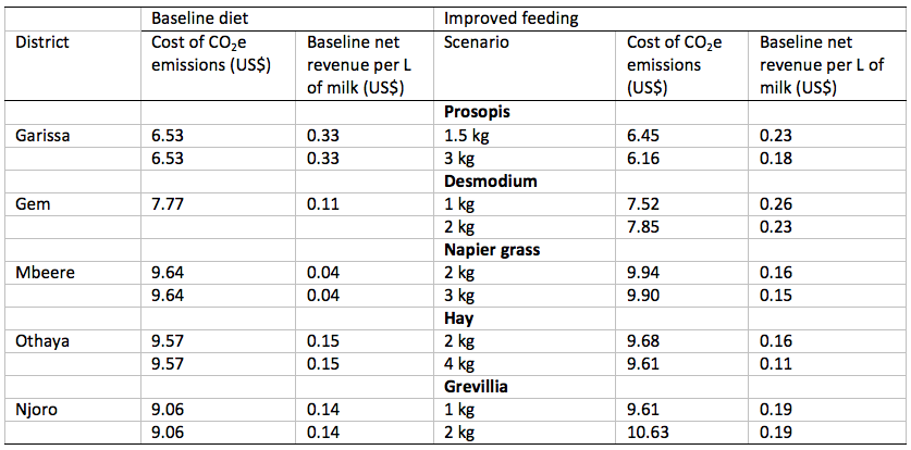
Empirical models are only one way to scale measured data. Process-based models are also used. For example, Bryan et al. (2013) averaged household data for seven counties and four agro-ecological zones in Kenya and used a process-based model to predict changes in methane emissions from enteric fermentation and revenue with improved feeding practices (Table 9.2). Process-based models consist of equations implementing current scientific understanding of the mechanisms determining system properties. Even though microbial and physicochemical processes involved in GHG emissions from soils are implemented in various biogeochemical models, equations are often based on empirical observations or represent apparent changes in production rates or microbial activity due to, for example, changes in environmental conditions such as changes in moisture and temperature. Thus, models describe a system consisting of components such as soil physics and energy fluxes, vegetation biomass development, or soil microbial C and N turnover and their interactions, which are represented by the equations describing states and rates at different points in time (temporal resolution). Process-based GHG models are designed to run at source scale (e.g., site or animal) after being calibrated based on observed relationships in controlled experiments and monitoring data. Because the equations represent principal microbial, biogeochemical and physicochemical processes underlying ecosystembatmosphere exchange processes and the emission of GHGs, the models can be suitable to simulate GHG dynamics under diverse environmental and management conditions, even conducting ‘what if’ scenario type of experiments. The robustness of process-based models has made them a widely used predictive tool in global change studies and they might be suitable as well to account for fine scale heterogeneity in the farming context, which is not possible with current empirical models. However, process-based models need to be tested for their ability to represent GHG under specific conditions to have confidence in their predictions. This is an involved process, which restricts their utility for sites and systems outside the range of the available calibration data. Until process-based models have been adapted, calibrated and evaluated to account for diversity and complexity characteristic of smallholder farming, their use for GHG quantification at the whole-farm level in mixed systems, such as the cropblivestock systems of Africa, remains a challenge, requires a tight coupling of sectorial models and a whole system understanding, and implies significant uncertainty.
The accuracy of a process-based model is related to errors due to model structure (model parameter uncertainty) or errors due to the accuracy of data inputs (input uncertainty). Errors related to model structure are based on incomplete understanding and knowledge of the fundamental relationships that are driving GHG production and consumption processes in soils, variation in ways to describe underlying processes, and fluxes at the soil-atmosphere interface and the representation of them in the model. These errors can be quantified statistically by comparing the model’s predicted GHG fluxes to measured GHG fluxes, with correlation coefficients for instance. Errors related to input uncertainty occur because the input data describing a particular system is not well known. This may be particularly problematic in developing countries when the detailed climate, soils, and land use data are not available at a high degree of resolution. Input uncertainty can be estimated using Bayesian calibration and Monte Carlo simulations (see for example Van Oijen et al. 2011; Rahn et al. 2011).
Table 9.2 Geographically averaged input data was used to run a process-based model (RUMINANT) to predict changes in emissions and revenues with changing diets under two scenarios.
Process-based models are available for the majority of biological GHG sources and sinks but tend to be limited to one type of source or sink. For instance, CENTURY, DAYCENT and LandscapeDNDC (Giltrap, Li, and Saggar 2010; Haas et al. 2013) were developed to simulate biomass production and soil processes, including simulation of soil GHG fluxes and soil C/N stock changes. Processbbased models are also available to simulate CH4 emissions from livestock but have so far mainly been applied in the US and in Europe (Thornton and Herrero 2010; Rotz et al. 2012; Duretz et al. 2011). These models are reasonable when evaluating the soil carbon sequestration potential at large scales or emissions of N2O from monoculture fields (Babu et al. 2006), or changes in herd management (Pathak et al. 2005; Bryan et al. 2013; Perlman et al. 2013) but perhaps less so when trying to characterize the GHG impacts of smallholder systems at the whole farm level or for landscape scale accounting.
Smallholder farming systems comprise multiple types of farming activities, often combining trees, animals, and crops in interconnected systems. Human management alters nutrients flows, potentially mitigating or exacerbating emissions from parts of the system; applying sectoral process-based models to whole farms therefore may oversimplify the complex interactions taking place (Tittonell et al. 2009). As of yet, few modeling approaches have been adapted for farm-level modeling of GHG impacts in mixed crop-livestock systems (Schils et al. 2007; Groot et al. 2012; Del Prado et al. 2013) and to our knowledge none have been applied to smallholder conditions of tropical developing countries.
To facilitate the widespread use of process-based models, as a first step the models need to be tested for most locations dominated by smallholder farming, which requires the availability of respective test datasets. Data on site-specific factors such as soil properties, cropping sequences, and fertilizer use are required; information which is often unavailable in many developing countries. In terms of enteric fermentation, the challenge is both a lack of information on animal numbers, species and breeds, feeding regimes, as well as the quality of feeds and forages even though the models are based on the presumption that the chemical reactions that occur in the rumen are fairly standard and tend to go to completion. However, emission factors and rates currently available which have been obtained so far (e.g. Bryan et al. 2013), don’t consider that livestock production in developing countries often involves periods of severe under nutrition with feed qualities being far lower than tested in experiments in OECD countries. It is obvious that there is a great need to generate data that can be used for model parameterization and evaluation for smallholder conditions. Until now, only limited information has been available to independently assess the validity of the emissions models for developing country conditions, casting doubt on the reliability of results generated from process-based models.
9.4 Conclusion
The complexity and scale that is characteristic of smallholder farming and the general lack of data presents significant challenges for scaling GHG emissions with much certainty. Significant efforts and investments are needed to improve systems representation so that the data collected are used to improve either empirical or process-based models. Moreover, conducting detailed monitoring campaigns can address the challenge of complexity and heterogeneity, and provide data that can be used to scale up representative systems with greater confidence.
Besides concerns over accuracy, technical demands in terms of data availability and model testing all limit the utility of using process-based models as a scaling method for GHG fluxes in agricultural systems of tropical developing countries at this time. However, given the costs of monitoring programs, it becomes an imperative to establish programs that can adapt and improve process-based models for quantification as they provide a means to test hypotheses of mitigation options and GHG accounting. This will require a number of investments in monitoring of smallholder practices of field and livestock management, scientific capacity building, and GHG measurements to evaluate the models for smallholder conditions. We estimate that a 10b year program of targeted and iterative measurements and modeling—those for key sources and sinks spanning heterogeneous conditions—is needed before use of process-based models becomes a viable solution for widespread GHG quantification in smallholder systems at either farm or landscape scales. In the meantime, models can be parameterized and tested well for farm and landscape situations, albeit time and resource intensive, but the limitations need to be recognized by those using the models and more importantly those using the model outputs.
Author affiliations
Corresponding author: Todd S. Rosenstock, World Agroforestry Centre, PO Box 30677O00100, UN Avenue-Gigiri, Nairobi, Kenya, t.rosenstock@cgiar.org, +254 20 722 4838
1 World Agroforestry Centre (ICRAF), Nairobi, Kenya
2 Lancaster Environment Centre, Lancaster University, formerly Center for International Forestry Research (CIFOR), Nairobi, Kenya
3 International Center for Tropical Agriuculture (CIAT), Cali, Colombia
4 Wageningen University and Research Centre, Wageningen, Netherlands
5 International Livestock Research Institute, Nairobi, Kenya
References
Del Grosso SL, Wirth T, Ogle SM, Parton WJ (2008) Estimating agricultural nitrous oxide emissions. EOS, Trans Am Geophys Union 89(51): 529b540
Groot JCJ, Oomen GJM, Rossing WAH (2012) Multibobjective optimization and design of farming systems. Agr Syst 110: 63b77
Holling CS (1992) Crossbscale morphology, geometry, and dynamics of ecosystems. Ecol Monogr 62(4): 447b502
Richards M et al. (in review) Limits of Greenhouse Gas Calculators to Predict Soil Fluxes in Tropical Agriculture. Sci Rep
Sieber S, AmjathbBabu TS, Jansson T, Müller K, Tscherning K, Graef F, Pohle D, Helming K, Rudloff B, SaraviabMatus BS, Gomez y Paloma S (2013) Sustainability impact assessment using integrated metabmodeling: Simulating the reduction of direct support under the EU common agricultural policy. Land Use Policy 33, 235b245
Stehfest E and Bouwman L. N2O and NO emissions from agricultural fields and soils under natural vegetation: summarizing available measurement data and modeling of global annual emissions. Nutri Cycl Agroecosyst 74(3):207b228
Van Groenigen JW, Velthof GL, Oeneme O, Van Groenigen KJ, Van Kessel C (2010) Towards and agronomic assessment of N2O emissions: a case study for arable crops. Eur J Soil Sci 61:903b913